This post is adapted from a short talk that I gave a couple years ago at Mathcamp. It’s intended for a general mathematically curious audience.
Introduction
Imagine you’re standing on a sphere at the north pole. Walk directly south until you get to the equator, then turn left. Walk along the equator until you’ve traced out of longitude, and then turn left again, so that you’re heading north. When you get back to the north pole, the path you’ve traced will look like Figure 1. Notice that this path you followed forms a triangle with three right angles.
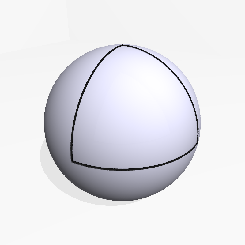
This would definitely be impossible if the world were flat — the only reason we’re able to draw a triangle with three right angles on the surface of a sphere is that it has what geometers call curvature. These notes are all about curvature, and what it can tell us about the geometry and topology of a surface. Almost all of the ideas we’ll discuss have analogues for smooth surfaces like the sphere, but we’re going to be investigating curvature on polyhedra, which are surfaces made from gluing together polygons along their edges and vertices.
Curvature and triangles
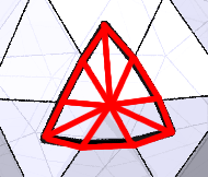
We can draw a similar picture on the surface of a cube rather than a sphere; it’s shown in Figure 2. You might initially be skeptical of our use of the word “triangle” for this shape. After all, it seems to have six edges rather than three. But there is a sense in which the lines that wrap around the edges of the cube are straight: if we took just the two faces of the cube that touch that edge, we could unfold them to form a flat rectangle, and after we did that our line would indeed be straight.
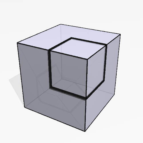
This will always be what we mean when we talk about polygons on the surface of a polyhedron. The lines that make up the edges — lines like the ones in Figure 2 that enter and exit each edge of the polyhedron at the same angle — are called geodesics, and they’re the closest analogue to straight lines we can find on the surface of a polyhedron: like straight lines in a plane, they form the shortest paths between any two nearby points lying along them.
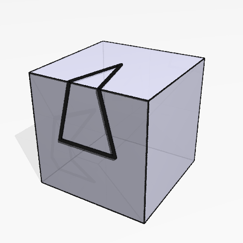
Once again, we see that it has three right angles, adding up to , more than we would get from drawing the same picture in a flat plane. Moreover, the extra seems to be specifically the fault of the corner: if you draw a triangle like in Figure 3, you can see that the angles sum up to the usual . In fact, if you tear off just the two faces of the cube that have the triangle on them, you can unfold them to make the triangle lie flat in a plane.
So there’s something going on at the corners of the cube that isn’t happening anywhere else, something that pushes out on these triangles, increasing the measures of their angles. We’ll say that the cube has curvature at its eight vertices, and is flat everywhere else.
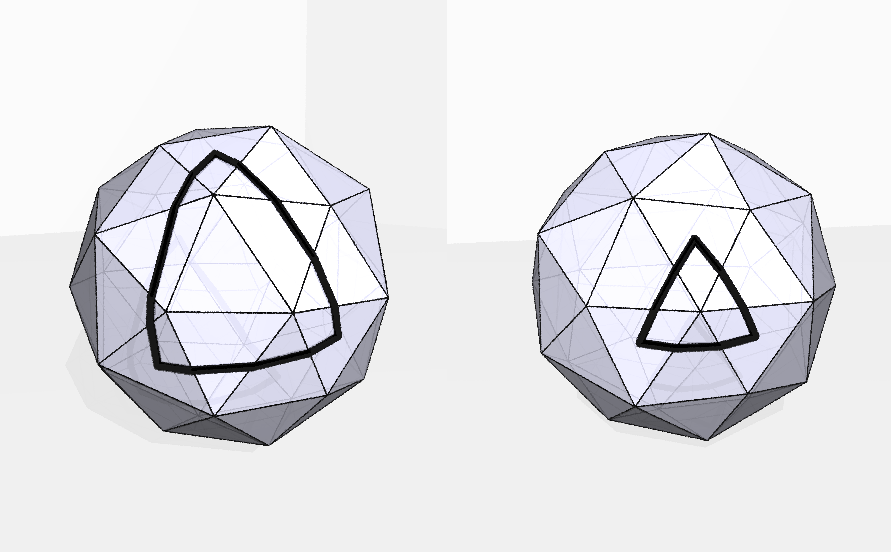
Furthermore, there’s a sense in which the cube has “ worth of curvature” sitting at each of its vertices: a triangle enclosing one of these vertices seems to get added to the sum of its angles. If we used another polyhedron instead of a cube, we might get a different number: the sum of the angles in the triangle on the right in Figure 4 is more than , but not a whole lot more; the triangle on the left looks a lot more like the one in our first example, and the sum of its angles is clearly quite a bit larger.
Angle deficit
Putting all this together, we seem to have arrived at a way to quantify curvature: draw a little triangle around a vertex, add up its angles, subtract , and that’s how much curvature that vertex has. But this leaves open a big question: if we’re trying to say that the amount of curvature at a vertex is just a property of that vertex and not a property of the triangle we chose to measure it with, then it had better be true that any triangle we use will give us the same answer.
In fact, this is true. One way to see it is to take a triangle that’s wrapped around a single vertex and cut it up into smaller triangles like in Figure 5: draw a line from the vertex to the triangle along each edge of the polyhedron, and also connect it to the vertices of the triangle.
Let’s suppose there are such triangles. (In the picture, .) We’d like to relate the sum of the angles of the triangle to something related to just the vertex itself. With this in mind, write for the sum of the angles of the triangle, and for the sum of the angles around the vertex. Then, on the one hand, the sum of the angles of all triangles is . On the other hand, we have lines touching an edge of the triangle and, since the edges of the triangle are geodesics, the angles at those points each add up to . So we get that
so
Now, we were trying to get an expression for how much extra angle we have in the triangle, that is, for . And we’re in luck: rearranging this last equation gives us that
That is, the amount that gets added to the angle sum of a triangle is the same as the difference between and the sum of the angles at the vertex. This number, , is called the angle deficit at the vertex, and this is the number we want to attach to a vertex to measure its curvature. Note that if the vertex is flat, then the sum of the angles at that vertex will be , making both sides of the equation zero, as expected.
What if the sum of the angles around a vertex is more than ? In that case, is negative, and so we say that that vertex has negative curvature. An example of this is shown in Figure 6. The vertex that the triangle is drawn around has five right angles at it, so the sum of its angles is , giving it a curvature of . So we should expect the sum of the angles of the triangle to add up to , and indeed the triangle in the picture has three angles.
The Gauss-Bonnet Theorem
In this last section, we’re going to talk about something remarkable that happens when you add up the curvatures for every vertex in a polyhedron. The number you get when you do this is called the total curvature. Now that we have the angle deficit description of the curvature at a vertex, the total curvature is fairly easy to compute. We can do it pretty quickly for all of the Platonic solids, pictured in Figure 7.
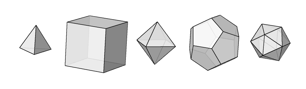
The results are:
| solid | vertices | faces at vertex | curvature at vertex | total curvature |
| tetrahedron | 4 | 3 triangles | ||
| cube | 8 | 3 squares | ||
| octahedron | 6 | 4 triangles | ||
| dodecahedron | 20 | 3 pentagons | ||
| icosahedron | 12 | 5 triangles |
Something should jump out right away: we always get the same number for the total curvature! In fact, there’s a deep reason for this, called the Gauss-Bonnet Theorem, which we’re about to prove.
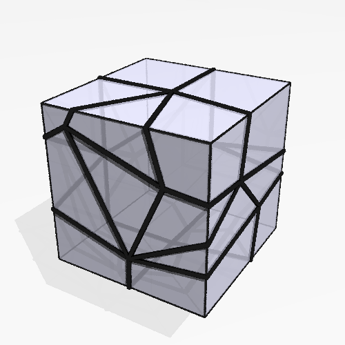
To prove this result, we’ll first need to triangulate our polyhedron, that is, cover it with triangles so that any two triangles meet at an edge and any two edges meet at a vertex. For this proof, we’re also going to require that none of the vertices of the triangles lies on top of a vertex of the polyhedron. A possible triangulation of a cube is shown in Figure 8.
The Gauss-Bonnet Theorem will give us a relationship between the total curvature and the shape of the triangulation we chose. We’re going to add up the angles of all the triangles in our triangulation, and just like when we proved the angle deficit formula in the last section, our result will come from counting the sum in two different ways.
Suppose our triangulation has vertices, edges, and triangles. (It’s important to remember that the vertices, edges, and triangles we’re talking about now are not the vertices, edges, and faces of the polyhedron itself!) Write for the total curvature of the polyhedron. On the one hand, when we add up all the angles inside all the triangles, we get , since the vertices of the triangles all lie at points with no curvature. On the other hand, we know that the sum of the angles of each triangle is plus the curvature inside it. All the vertices of the polyhedron are inside some triangle, so altogether we’re going to get : for each triangle, plus all the adjustments we have to make to account for the curvature.
Putting these together, we see that
so
We should pause here to take stock of what we just proved. The left-hand side of that formula has nothing to do with the triangulation we chose; it’s just the sum of the curvatures at each vertex of the polyhedron. But the right-hand side is the opposite: it’s only about the triangulation, and it has nothing to do with the geometry of the polyhedron we drew it on. So no matter what triangulation you use for a polyhedron, is always the same number. And if we’re able to wrap the same triangulation around two different polyhedra, then those two polyhedra must have the same total curvature. It’s this last result that tells us why we saw what we did for the Platonic solids: it’s easy to see that any triangulation that works for one of them will work for any of the others. (For example, you could put the two Platonic solids on top of each other so they’re both centered at the same point, and project the vertices of the triangulation out from one of them onto the other.)
The number is called the Euler characteristic of the triangulation, and it’s usually written in a different form, . In fact, since we only used triangles, these two numbers are the same. To see this, notice that you can count the edges of the triangulation by multiplying the number of triangles by 3; each triangle has three edges, so every edge is accounted for. But this counts each edge twice, since each edge shows up for exactly two of the triangles. So , that is, , so
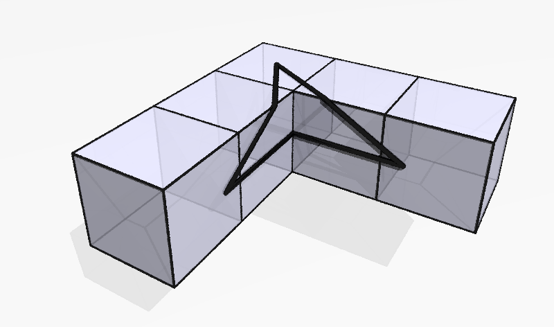
Does the Gauss-Bonnet Theorem mean that every polyhedron has the same total curvature? Consider the polyhedron in Figure 9.
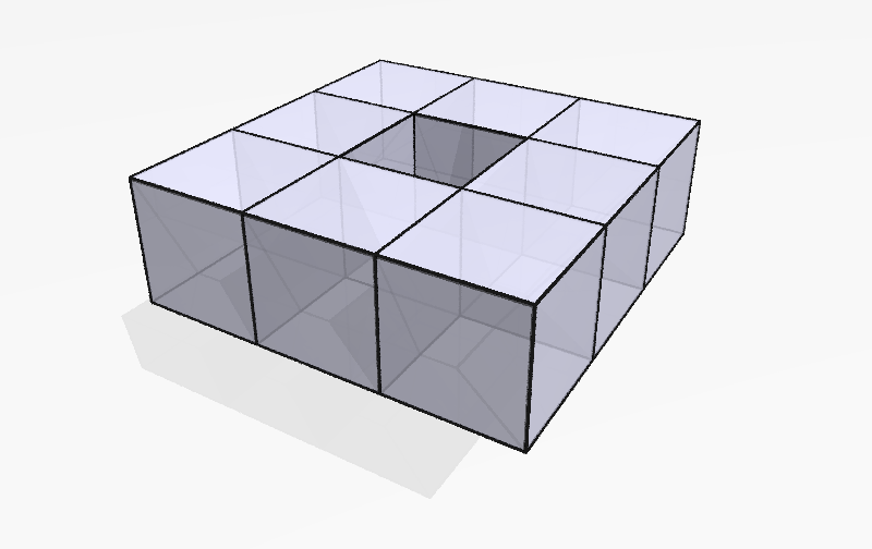
It has eight vertices on the outside with three right angles, which give a curvature of each, and eight vertices on the inside with five right angles, which give a curvature of each. So the total curvature is 0, which is a different number than we got for the Platonic solids. By Gauss-Bonnet, this means that the Euler characteristic of any triangulation of this thing is also 0. This is, perhaps not surprisingly, because of the hole in middle: if we tried to use one of the triangulations that worked before, we would find that some of the edges would need to go across the hole.
Mathematicians like to say that the Euler characteristic depends only on the “topology” of the polyhedron and not on its “geometry.” The topology of the polyhedron, roughly speaking, consists of those properties that don’t change when we continuously deform it, pushing vertices outward or inward, making dents or bubbles, or anything else that doesn’t require us to tear or glue the surface. A triangulation is indifferent to these sorts of changes: if a face of the polyhedron moves around slightly, we can nudge the lines in our triangles accordingly. This, of course, breaks down if we have to tear a hole like in Figure 9: this might cut an edge of the triangulation, and there’s no obvious way to reattach it.
This is what makes Gauss-Bonnet so remarkable. It gives us a relationship between geometry — in the form of the curvatures at each of the vertices — and topology — in the form of the triangulation — two different aspects of our surface that would seem not to have a lot to do with each other. This is the type of result that mathematicians crave; whenever we see a connection between two seemingly distant fields, it’s a sign that there’s much more depth there to explore.