Introduction

This article is the third in a series on physics for mathematicians. This series contains a later article on gauge fields, and I plan to also produce one on general relativity, and as the plans for those two topics came together I decided it would be helpful if I first covered an important piece of machinery that they both have in common.

The object we will be discussing is called a “connection.” Roughly speaking, a connection is an extra piece of structure that can be put on a fiber bundle that allows you to compare nearby fibers with each other. This topic is a standard part of many differential geometry textbooks, but I am taking a somewhat unorthodox approach, starting out from a more general perspective than usual. I’ve done this for two reasons. First, the discussion of gauge theory needs the more general version anyway, and it might be preferable to avoid repeating the work needed to get there. But second, and more importantly, the common special cases — especially the case of connections on the tangent bundle — make more sense when one knows what a connection is supposed to look like in other settings.

The prerequisites for following this presentation are similar to those for the article on Hamiltonian and Lagrangian mechanics. The target audience (if such a person exists at all) is someone who is reasonably comfortable with the fundamental ideas of differential geometry, including fiber bundles and vector bundles, the Lie bracket of vector fields, the definition of a Riemannian metric, and Stokes’ Theorem, but who doesn’t know how to define curvature, and who might not know what connections are or why anyone would care about them.

Every topological space appearing in this article is a smooth manifold. If \(M\) is a manifold, we’ll write \(TM\) for its tangent bundle and \(T_xM\) for the tangent space at some point \(x\in M\). Given a map \(f:M\to N\) of manifolds, we will write \(f_*:T_xM\to T_{f(x)}N\) for the induced map on tangent spaces. Similarly, we will spend a lot of time talking about fiber bundles of the form \(\pi:E\to M\), and we will often use the notation \(E_x\) to refer to the fiber \(\pi^{-1}(\{x\})\). Given a Lie group \(G\) and some \(g\in G\), we will use the common convention of writing \(L_g:G\to G\) for the map defined by \(L_g(h)=gh\), and similarly for \(R_g\).

One of the most enjoyable aspects of writing this article was the chance to solidify my own knowledge of the material, and I found several sources helpful, including:

• A Comprehensive Introduction to Differential Geometry by Michael Spivak, especially Volume II.
• Gauge Fields, Knots, and Gravity by John Baez and Javier P. Muniain
• Global Calculus by S. Ramanan
• Natural Operations in Differential Geometry by Ivan Kolář, Peter W. Michor, and Jan Slovák (available on Michor’s website)

I’m very grateful to Yuval Wigderson, Hunter Brooks, Jake Levinson, and Jeff Hicks for reading through and commenting on earlier versions of this article.

Dragging Things in Fiber Bundles

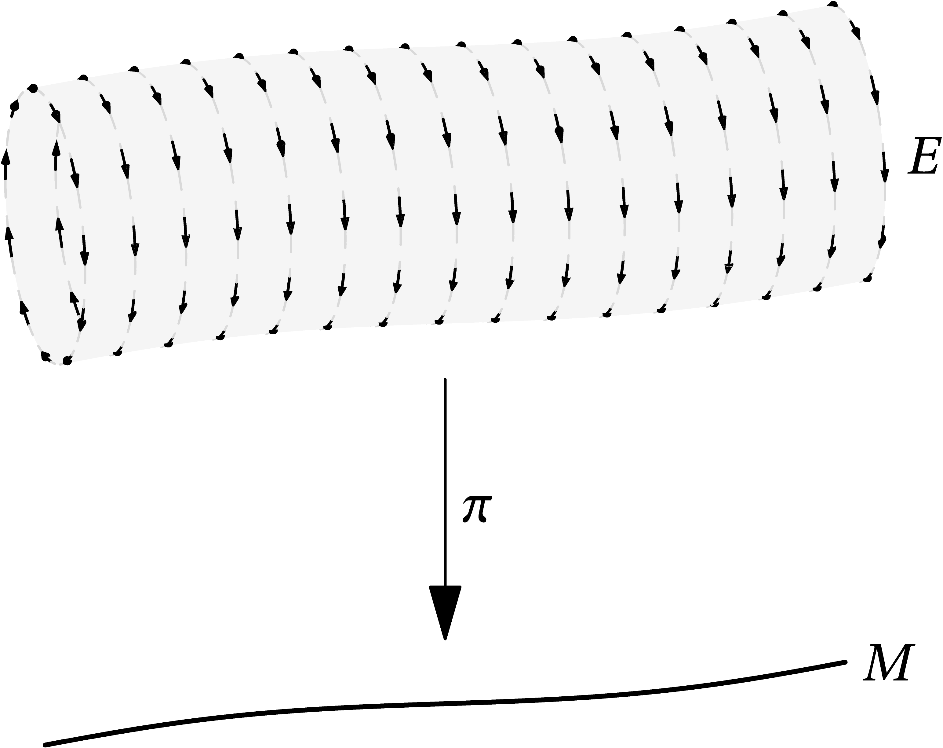
Consider a fiber bundle \(E\) over a manifold \(M\), and write \(\pi:E\to M\) for the projection. The usual intuition is that a point \(e\in E\) is meant to represent a choice of some extra piece of data we are attaching to the point \(\pi(e)\in M\). For example, if \(E\) is the tangent bundle of \(M\), then \(e\) represents the point \(\pi(e)\) together with a choice of tangent vector at that point.

Throughout this article we will be concerned with one particular thing one might want to do with such a piece of data. Suppose we have a path \(\gamma:[0,1]\to M\) starting at \(\pi(e)\). How can we “drag” the extra piece of data we’ve chosen (the tangent vector, say) along \(\gamma\) from \(\gamma(0)=\pi(e)\) to \(\gamma(1)\)? This procedure (once we have been told how to do it) is called “parallel transport.”

There are many settings in which a notion of parallel transport arises naturally, and we are about to consider a couple examples. But the structure of the fiber bundle alone is not enough to give us a rule for parallel transport — while each fiber can be identified with some standard fiber \(F\), in general there is no canonical way to do this, and therefore no way to declare that, say, a tangent vector at one point is “the same tangent vector” as one at another point. We will therefore need to add an extra piece of structure to the fiber bundle in order to know how parallel transport is supposed to work. This extra piece of structure is called a “connection,” and it’s what this article is all about.

Motivating Examples

In an attempt to make the definition of connection we land on seem as intuitive as possible, we will build it up in steps by considering two examples in which parallel transport arises naturally.

Example 1. Imagine a spherical marble rolling around on a planar table. We will assume there is enough friction that the marble never “spins or slips,” so that when we push it in some direction it rolls about the perpendicular axis:

Our goal is to find a way to describe, for any path \(\gamma\) in the plane, how the marble rotates as we roll it along \(\gamma\).

We can specify the configuration of the marble at any moment in time with two pieces of information: the point of the plane that the marble touches, and how the marble is oriented above that point. By embedding the whole picture in \(\mathbb{R}^3\), so that the plane is the \(x\)-\(y\) plane and the marble sits directly on top of it, the configuration of the marble can be given by an element of \(SO(3)\), and so the whole configuration space can be identified with the trivial fiber bundle \(\mathbb{R}^2\times SO(3)\) over \(\mathbb{R}^2\). We’ll write \(\pi:\mathbb{R}^2\times SO(3)\to\mathbb{R}^2\) for the projection map.

We can then phrase the “how to roll” problem in terms of this fiber bundle: given a point \(e\in \mathbb{R}^2\times SO(3)\) and a path \(\gamma:[0,1]\to\mathbb{R}^2\) starting at \(\pi(e)\), how should we lift \(\gamma\) to a path \(\widetilde\gamma:[0,1]\to \mathbb{R}^2\times SO(3)\) so that \(\widetilde\gamma(0)=e\), \(\pi(\widetilde\gamma(t))=\gamma(t)\) for all \(t\), and the lifted tangent vector indicates which direction the marble rolls? Once we have a rule for producing \(\widetilde\gamma\) from \(\gamma\), the \(SO(3)\) part of \(\widetilde\gamma(t)\) will tell us how the sphere is rotated after it has been rolled along the path up to \(\gamma(t)\).

Example 2. Consider a manifold \(M\) embedded in some \(\mathbb{R}^n\), and take a point \(x\in M\) and a tangent vector \(v\in T_xM\). For any path \(\gamma:[0,1]\to M\) starting at \(x\), we would like a way to produce a tangent vector at each \(\gamma(t)\) which is, in some suitable sense, the result of dragging \(v\) along the path up to that point. In other words, writing \(\pi:TM\to M\) for the projection, we are looking for a way to lift \(\gamma\) to a path \(\widetilde\gamma:[0,1]\to TM\) with \(\widetilde\gamma(0)=v\) and \(\pi(\widetilde\gamma(t))=\gamma(t)\) for all \(t\).

There is of course no canonical way to choose \(\widetilde\gamma\) given just the manifold \(M\), but the embedding of \(M\) into \(\mathbb{R}^n\) produces a natural choice. The embedding also lets us embed tangent vectors to \(M\) into \(\mathbb{R}^n\), and this second embedding allows us to ask how the tangent vectors \(\widetilde\gamma(t)\) are changing as we move along \(\gamma\), that is, it gives meaning to the expression \((d/dt)\widetilde\gamma(t)\in\mathbb{R}^n\). We then declare that the vectors \(\widetilde\gamma(t)\) are parallel transported along \(\gamma\) if this derivative is always orthogonal to the tangent space at \(\gamma(t)\):

We can think of this condition as asking for the tangent vectors to “change as little as possible” as we move along \(\gamma\); the vectors are forced to “bend” in the directions perpendicular to \(M\) just to remain tangent to \(M\), and we say they are parallel transported if they do not bend any more than this.

Fiber Bundle Connections

The Definition

In both cases, we seek a rule for lifting a path on a manifold up to a fiber bundle. It’s possible to describe connections directly in terms of such a rule, but, like so many constructions in differential geometry, it turns out to be much cleaner to start with the “infinitesimal” version — a way to lift tangent vectors rather than paths — and build a path-lifting rule out of that. So, given a fiber bundle \(\pi:E\to M\), a point \(e\in E\), and a tangent vector \(v\in T_{\pi(e)}M\), we want a way to pick a tangent vector \(\widetilde v\in T_eE\) so that \(\pi_*(\widetilde v)=v\).

A tangent vector \(v\in TE\) is called vertical if \(\pi_*(v)=0\). (The picture to have in mind is that vertical tangent vectors “point along the fibers” of the bundle.) We will write \(VE\subseteq TE\) for the subbundle consisting of the vertical vectors. There is no canonical way to define “horizontal” tangent vectors just using the fiber bundle structure; any local trivialization of \(E\) will give you a way to do it, but different choices of trivialization will give different ones. A fiber bundle connection on \(E\) is exactly such a choice: it is a vector subbundle \(HE\subseteq TE\) for which, at each point \(e\in E\), the projection \(\pi_*|_{H_eE}:H_eE\to T_{\pi(e)}M\) is an isomorphism. (This is equivalent to requiring that \(HE\) is complementary to \(VE\), i.e., that \(T_eE=V_eE\oplus H_eE\) at each \(e\).) Given a connection, tangent vectors in \(HE\) are called horizontal.

This is exactly what we need in order to lift tangent vectors: since \(\pi_*|_{H_eE}\) is an isomorphism for each \(e\in E\), we can invert it to take any tangent vector \(v\in T_{\pi(e)}M\) to a tangent vector \(v^*_e\in H_eE\), which we will call the horizontal lift of \(v\) to \(e\). We will frequently go back and forth between the “horizontal subspace” and “horizontal lift” definitions of connections.

We will also frequently use the direct sum decomposition to split a vector \(v\in T_eE\) into its horizontal part \(v^H\in H_eE\) and its vertical part \(v^V\in V_eE\). Note that, even though the vertical subspace is well-defined without choosing a connection, we can’t take the vertical part of a vector without one.

Given a path \(\gamma:[0,1]\to M\), we say that a path \(\widetilde\gamma:[0,1]\to E\) is a horizontal lift of \(\gamma\) if, for all \(t\),

• \(\widetilde\gamma'(t)\in H_{\gamma(t)}E\), and
• \(\pi_*(\widetilde\gamma'(t))=\gamma'(t)\).

Under any choice of coordinates, these two conditions are equivalent to a system of ordinary differential equations. This means that a fiber bundle connection on \(E\) at least lets us lift paths locally, that is, for each \(t\) we can find a unique \(\widetilde\gamma:(t-\epsilon,t+\epsilon)\to E\) satisfying these properties for some \(\epsilon\). If we can always lift the entire path we say that the connection is complete. While not every fiber bundle connection is complete, all of the connections we will actually spend any time considering in this article will be, including both of the examples discussed so far, so we will not spend much time worrying about it.

Given a complete connection, we can take a path \(\gamma:[0,1]\to M\) and a point \(e\in E_{\gamma(0)}\) and produce a unique horizontal lift \(\widetilde\gamma\) with \(\widetilde\gamma(0)=e\). We will say that the point \(\widetilde\gamma(1)\in E_{\gamma(1)}\) is the result of parallel transporting \(e\) along \(\gamma\). Because it was defined in terms of solutions to ODE’s, it is straightforward to check that reparametrizing \(\gamma\) doesn’t affect the result of parallel transport and, in particular, if \(\gamma^{\mathrm{rev}}(t)=\gamma(1-t)\) is the reversal of \(\gamma\), then \(e\) is also the result of parallel transporting \(\widetilde\gamma(1)\) along \(\gamma^{\mathrm{rev}}\).

The Examples

Both of the “dragging procedures” we’ve described so far — the rolling marble and parallel transport of tangent vectors on an embedded manifold — can be described as fiber bundle connections.

In the case of the rolling marble, we want a connection on the trivial fiber bundle over \(\mathbb{R}^2\) with fiber \(SO(3)\). The fact that the fiber bundle in question is trivial gives an obvious way to lift a tangent vector: if \(e=(x,g)\in \mathbb{R}^2\times SO(3)\) and we are given \(v\in T_x\mathbb{R}^2\), we could just let the horizontal lift be \((v,0)\in T_x\mathbb{R}^2\times T_g SO(3)=T_e(\mathbb{R}^2\times SO(3))\). But this corresponds to sliding the marble across the plane so that it never rotates, which is not what we want! The lifting prescription that corresponds to the rolling we’re after will have to be something else.

We’ll start by lifting tangent vectors from a point \(p\in\mathbb{R}^2\) to \((p,1)\in \mathbb{R}^2\times SO(3)\), where 1 means the identity element. Suppose we want to lift \(\partial_x\in T_p\mathbb{R}^2\), the tangent vector pointing in the positive \(x\) direction. Pushing the marble in this direction makes it rotate counterclockwise about the positive \(y\) axis, that is, using a right-handed coordinate system, in the direction that moves the positive \(z\) axis toward the positive \(x\) axis. This rotation is generated by the element we’ll call \[r_x=\begin{pmatrix}0&0&1\\0&0&0\\-1&0&0\end{pmatrix}\in T_1SO(3)=\mathfrak{so}(3),\] so \((\partial_x)^*_{(p,1)}=(\partial_x,r_x)\). (Depending on the radius of the marble, there ought to be a coefficient in front of this matrix, but let us assume for simplicity that it’s 1.) Similarly, \[r_y=\begin{pmatrix}0&0&0\\0&0&1\\0&-1&0\end{pmatrix}.\]

So the horizontal subspace \(H_{(p,1)}(\mathbb{R}^2\times SO(3))\) is spanned by the vectors \((\partial_x,r_x)\) and \((\partial_y,r_y)\), and we can lift an arbitrary vector \(v=\alpha\partial_x+\beta\partial_y\) to \((v,\alpha r_x+\beta r_y)\). What about at points other than the identity in \(SO(3)\)? Whatever configuration of the marble is represented by \(1\), a point \(g\in SO(3)\) represents the configuration resulting from applying \(g\) to it. If we were to then rotate the marble again using some \(h\in SO(3)\), the resulting configuration would of course be represented by \(h\cdot g\); in this sense \(SO(3)\) acts on the marble on the left. So, if we start at the configuration \(g\) and push the marble in \(\partial_x\) direction, then, starting at the identity, we have first performed \(g\), and then performed a small rotation in the \(r_x\) direction. So the vector we want is \(r_x\cdot g=(R_g)_*(r_x)\). (The expression on the left has meaning only as a matrix; since \(R_g\) acts linearly on the coefficients of a matrix in \(SO(3)\), its action on tangent vectors is the same linear map.)

We’ll next consider the second example about dragging tangent vectors on an embedded manifold. Since tangent vectors are the things we intend to drag around \(M\), we need a connection on \(TM\), that is, a choice of horizontal subspace in each tangent space of the tangent bundle. It is easy to get confused here! We are looking at \(T(TM)\), and the two \(T\)’s appear for two different reasons: the innermost \(TM\) is here because this is the bundle on which we are trying to define the connection, but the outermost \(T\) would be there regardless — connections are always “about” tangent vectors in this second sense.

We’ll start by giving a more explicit description of \(T(TM)\) when \(M\) comes with an embedding in \(\mathbb{R}^n\). Suppose \(\dim M=n-d\), so that \(M\) is locally cut out by equations \(f_\alpha(x)=0\) for \(\alpha=1,\ldots,d\). As we said before, we can use our embedding to think of tangent vectors as also living in \(\mathbb{R}^n\); if we do this, then \((x,v)\in\mathbb{R}^n\times\mathbb{R}^n\) lives in \(TM\) if and only if, for each \(\alpha\), \[\text{(a) }f_\alpha(x)=0,\qquad\text{(b) }(\partial_vf_\alpha)(x)=0.\]

To determine when some \((w,\eta)\in\mathbb{R}^n\times\mathbb{R}^n\) is tangent to \(TM\) at \((x,v)\) we have to differentiate both sets of equations (a) and (b). (Again, the two tangent vectors \(v\) and \(w\) appear for two different reasons: \(v\) is the vector we are attempting to drag, \(w\) is the direction in which we want to drag it, and \(\eta\) represents the change in \(v\) that might or might not constitute parallel transport.) From (a) we get that \((\partial_wf_\alpha)(x)=0\), i.e., \(w\) is also tangent to \(M\); since the original equation doesn’t involve \(v\), this new one doesn’t involve \(\eta\). Differentiating (b) gives us \[(\partial_v\partial_w f_\alpha)(x)+(\partial_\eta f_\alpha)(x)=0.\]

The thing to notice here is that, if we write \(\eta=\eta^\perp+\eta^\parallel\) with \(\eta^\parallel\in T_xM\) and \(\eta^\perp\) orthogonal to \(T_xM\), then this last condition determines \(\eta^\perp\) completely for a given \(x\), \(v\), and \(w\); in fact, the numbers \((\partial_\eta f_\alpha)(x)\) can be used as coordinates for \((T_xM)^\perp\). We referred earlier to the fact that, in order for a moving tangent vector to stay tangent to \(M\), it has to move perpendicular to \(M\). Since \(\eta\) represents a change in \(v\), \(\eta^\perp\) is exactly this required perpendicular movement.

All of this so far just gives us the equations that cut out \(T(TM)\) in \(\mathbb{R}^n\times\mathbb{R}^n\times\mathbb{R}^n\times\mathbb{R}^n\). In order to express our parallel transport condition from earlier in terms of a connection, we need to say when some \((w,\eta)\in T_{(x,v)}(TM)\) ought to belong to the horizontal subspace; \(\eta\) represents the first-order change in \(v\) as we attempt to drag \(v\) in the \(w\) direction, and \((w,\eta)\) should be horizontal when this change in \(v\) coincides with our notion of parallel transport. Our condition was that the change in the parallel transported vector should be perpendicular to \(T_xM\), so our connection is defined by declaring that \((w,\eta)\in H_{(x,v)}(TM)\) if and only if \(\eta^\parallel=0\). Since \(\eta^\perp\) was already determined by our choice of \(x\), \(v\), and \(w\), this additional constraint completely determines \(\eta\). So, as must always be true for any connection, every \(w\in T_xM\) indeed has a unique horizontal lift up to the tangent space to any point \((x,v)\) in the fiber of \(TM\) over \(x\).

The resulting connection on \(TM\) depends crucially on the way we embedded \(M\) into \(\mathbb{R}^n\) — we used the embedding in order to talk about \(\eta\) at all, and we also used the metric on \(\mathbb{R}^n\) to split \(\eta\) into \(\eta^\perp\) and \(\eta^\parallel\). However, we will see later on that this connection is a bit less arbitrary than it might appear: it will turn out to depend only on the Riemannian metric on \(M\) that it inherits from the embedding, rather than on any other details of the embedding itself.

Connections and Structure Groups

The bundles we will be most interested in having connections on are \(G\)-bundles, and in particular it will be important to know what it means for a connection on a \(G\)-bundle to “respect the \(G\)-bundle structure.” The idea should be that, whatever the structure in the fiber is that \(G\) is meant to preserve, parallel transport ought to preserve it as well. (For example, for vector bundles, we want the parallel transport maps to be linear.)

Throughout this discussion we will move between two different ways of thinking about \(G\)-bundles: in terms of their transition functions and in terms of their associated principal bundles. In case any of this is unfamiliar, I’ve written a short supplement to this article going through how all the definitions work. Even a reader who is already comfortable with both of these perspectives might want to read the summary at the end of that supplement to see the notation and terminology I’ll be using here.

There are also several ways to describe the structure we are about to discuss, and in this section we will go through three of them: one coming from the description of a \(G\)-bundle in terms of transition functions and two coming from the associated principal bundle construction. Each is illuminating in its own way, so we will spend some time getting to know them all. This will, by necessity, be somewhat dry and technical; I’ve included a summary at the end of the section for any readers who might have gotten lost in the details.

Local Description

We start with a \(G\)-bundle \(\pi:E\to M\) with standard fiber \(F\) and a fiber bundle connection on \(E\). We’ll work for now with just one trivialization for our \(G\)-bundle, i.e., a diffeomorphism \(\phi:\pi^{-1}(U)\to U\times F\) for some open set \(U\subseteq M\). After making this choice, it is straightforward to say what we want from the parallel transport.

Given a path \(\gamma:[0,1]\to U\) and a point \(e\in E\), our connection gives us a horizontal lift \(\widetilde\gamma_e:[0,1]\to E\) for which \(\widetilde\gamma_e(0)=e\). Since the definition we are working towards is about what this parallel transport procedure does to \(e\), we introduce notation that emphasizes this, writing \(\operatorname{pt}_\gamma^t(e)=\widetilde\gamma_e(t)\). We’ll also write \(\phi_2:\pi^{-1}(U)\to F\) for the second coordinate of our trivialization \(\phi\), so that \(\phi(e)=(\pi(e), \phi_2(e))\).

We then say that our connection is a \(G\)-bundle connection if the action of parallel transport on the fibers always comes from the action of \(G\) on \(F\), that is, there is a map \(a_\gamma:[0,1]\to G\) so that, for each \(t\), \[\phi(\operatorname{pt}_\gamma^t(e))=(\gamma(t),a_\gamma(t)\cdot\phi_2(e)).\]

Note that, since the action of \(G\) on \(F\) is effective, such an \(a_\gamma\) is unique if it exists. It is important to emphasize that we want \(a_\gamma\) not to depend on \(e\): if, for example, we are working with vector bundles and \(G=GL(n)\), we want each \(\operatorname{pt}_\gamma^t\) to be a linear map, a condition which is independent of the point in the fiber we are applying the linear map to.

Of course, in order for this definition of \(G\)-bundle connections to be well-defined, we need to check that it doesn’t depend on the trivialization we used to write it down. Because we are working with \(G\)-bundles, any other trivialization \(\bar\phi:\pi^{-1}(U)\to U\times F\) differs from the one we started with by a map \(g:U\to G\), that is, \(\bar\phi(\phi^{-1}(x, f))=(x, g(x)\cdot f)\). Suppose our connection is a \(G\)-bundle connection according to the trivialization \(\phi\), so for any path \(\gamma\) we have a map \(a_\gamma\) as above. Then \[\begin{aligned} \bar\phi(\operatorname{pt}_\gamma^t(e))&=(\gamma(t),g(\gamma(t))a_\gamma(t)\cdot\phi_2(e))\\ &=(\gamma(t),g(\gamma(t))a_\gamma(t)g(\gamma(0))^{-1}\cdot\bar\phi_2(e)). \end{aligned}\] So in fact our connection is a \(G\)-bundle connection according to \(\bar\phi\) as well, because we can take \(\bar a_\gamma(t)=g(\gamma(t))a_\gamma(t)g(\gamma(0))^{-1}\) as the replacement for \(a_\gamma\) in the definition.

This proves that our definition is well-defined, but it’s still a bit inconvenient to work with. After all, we defined connections in terms of tangent vectors, so it would be nice to define \(G\)-bundle connections in a similar way. We can get what we want by differentiating the definition we just gave. Take a tangent vector \(v\in T_xM\) and a point \(e\) in the fiber of \(x\). If our connection is a \(G\)-bundle connection, then, imagining \(v=\gamma'(0)\) for some path \(\gamma\), we can differentiate our earlier description to see that our condition becomes \[\phi_*(v^*_e)=(v, -A(v)\cdot\phi_2(e)),\] where \(A(v)=-a_\gamma'(0)\in\mathfrak g\). (The minus sign is conventional; I’ll mention later why we include it.) Here we are following the convention of writing, for \(X\in\mathfrak g\) and \(f\in F\), \(X\cdot f=(\sigma_f)_*X\in T_fF\), where \(\sigma_f:G\to F\) is given by \(\sigma_f(g)=g\cdot f\).

I encourage you to verify that \(A\) depends linearly on \(v\). We call a map \(TM\to\mathfrak g\) which is linear on the fibers of \(TM\) a \(\mathfrak g\)-valued 1-form. It is the same as a map of vector bundles \(TM\to\mathfrak g\), where we follow the common convention of identifying a vector space with the corresponding trivial vector bundle. If we have a basis for \(\mathfrak{g}\), a \(\mathfrak g\)-valued 1-form can be thought of as just a list of ordinary 1-forms on \(M\), one for each coordinate.

Using this language, our connection is a \(G\)-bundle connection if and only if there is a \(\mathfrak g\)-valued 1-form \(A\) satisfying \(\phi_*(v^*_e)=(v, -A(v)\cdot\phi_2(e))\) for every \(v\) and \(e\). We proved one direction of this equivalence just now; for the converse, I encourage you to check that in fact any \(\mathfrak g\)-valued 1-form \(A\) gives rise to a connection according to this rule. Like our original definition, this one superficially depends on the trivialization we picked. While we already know that it doesn’t from the earlier discussion about parallel transport, it’s also worth seeing the coordinate change formula for \(A(v)\) explicitly, which you will do in the exercises.

It will be useful to have some notation for the way one recovers the parallel transport maps \(a_\gamma\) from \(A\). By the way \(A\) was constructed, \(a_\gamma\) satisfies the differential equation \[a_\gamma'(t)=-A(\gamma'(t))\cdot a_\gamma(t)\] with the initial condition \(a_\gamma(0)=1\). (Again, we write \(X\cdot g=(R_g)_*X\) for \(g\in G\) and \(X\in\mathfrak g\).) If \(a_\gamma\) were a real-valued function, or even a function taking values in an abelian Lie group, this equation would be satisfied by \(a_\gamma(t)=\exp\int_0^t-A(\gamma'(s))ds\).

Sadly, proving this in the abelian case requires using the fact that \(\exp(X+Y)=\exp X\cdot\exp Y\) for \(X,Y\in\mathfrak g\), which just isn’t true in general. Thinking of elements of \(\mathfrak g\) as transformations that are infinitesimally close to the identity, you can think about that exponential integral as aggregating all of these small transformations as we move across \(\gamma\). The problem in the nonabelian case then arises because it matters what order we perform them in! The differential equation prescribes this order.

This gives rise to a convention that is especially common in physics: we define the path-ordered exponential integral of \(-A\) along \(\gamma\) to be the solution to that differential equation, and we write \[a_\gamma(t)=\operatorname{Pexp}\int_0^t-A(\gamma'(s)).\] (To avoid confusion with this notation, it’s probably best to just think of “\(\operatorname{Pexp}\int\)” as a single symbol.) When every \(A(\gamma'(s))\) commutes with every other this coincides with the ordinary exponential integral. You’ll explore this object a bit more in the exercises.

Principal and Induced Connections

There is also a more “global” picture of \(G\)-bundle connections arising from the associated principal bundle construction. In our previous discussion, we wanted to require the parallel transport maps to come from the left \(G\)-action on the fiber, but this left \(G\)-action is only well-defined after choosing a trivialization, leading us to the somewhat roundabout definition we ended up with. But the situation is simpler for principal bundles: a map \(G\to G\) comes from the left action of \(G\) on itself if and only if it commutes with the right action of \(G\) on itself, and this right action extends to a well-defined right action on the entire principal bundle.

So, if \(P\) is a principal \(G\)-bundle over \(M\), a fiber bundle connection on \(P\) is a \(G\)-bundle connection if and only if the horizontal subbundle \(HP\subseteq TP\) is preserved by the right action of \(G\) on \(P\). These are called principal connections. In terms of individual horizontal subspaces, this means that, for \(p\in P\), \((R_g)_*(H_pP)=H_{p\cdot g}P\). In particular, the connection is fully determined once we have specified one of the horizontal subspaces in each fiber.

This is equivalent to asking for parallel transport to commute with the right action of \(G\). That is, given a path \(\gamma\) in \(M\), then we want lifting to a path starting at \(p\cdot g\in P\) to be the same as first lifting to a path starting at \(p\) and applying \(g\) pointwise along the lifted path. This is exactly what we want in a case like our rolling marble from the first section, where the action of \(G\) is a symmetry of the entire situation we are trying to model. The way the marble is rotated when you roll it along a path has nothing to do with which configuration you chose to call the “identity” at the start of the path.

This definition can be turned into a global description of all \(G\)-bundle connections, not just the principal ones. Let \(E\) be a \(G\)-bundle on \(M\) with fiber \(F\) and let \(P\) be its associated principal bundle. If we’ve chosen a principal connection on \(P\), there is a natural way to produce a \(G\)-bundle connection on \(E\). One example to keep in mind is to imagine how we could turn our rolling marble connection on \(\mathbb{R}^2\times SO(3)\) and the left action of \(SO(3)\) on \(S^2\) into a connection on \(\mathbb{R}^2\times S^2\) describing how the point of contact with the plane moves along the surface of the marble as we roll it.

We will start with the case of trivial bundles. (This is only for motivation; the definition we arrive at won’t actually depend on a choice of trivialization.) So let \(P\cong M\times G\) and \(E\cong M\times F\), and suppose we’re given a path \(\gamma:[0,1]\to M\). Using the principal connection on \(P\), lift \(\gamma\) to a path \[\widetilde\gamma(t)=(\gamma(t),\widetilde\gamma_2(t))\in M\times G,\] choosing the lift starting at \((\gamma(0),1)\). The points \(\widetilde\gamma_2(t)\in G\) give us a family of transformations of \(F\) starting at the identity, and we will use them to define our desired lifted path: we want a connection on \(E\) for which \(\gamma\) lifts to \[\widetilde\gamma'(t)=(\gamma(t),\widetilde\gamma_2(t)\cdot f)\in M\times F.\]

But, despite appearances, this condition doesn’t actually depend on the choice of trivialization. Recall that we can describe the \(G\)-bundle structure on any \(G\)-bundle \(E\) using an isomorphism \(E\cong P\times_GF\). There is a projection map \(\chi:P\times F\to P\times_GF\) sending each \((p,f)\in P\times F\) to its equivalence class under the relation \((p\cdot g,f)\sim(p,g\cdot f)\). In this language, the path lifting procedure we just described for trivial bundles is equivalent to using the connection on \(P\) and a constant path on \(F\) to lift \(\gamma\) all the way up to \(P\times F\) and then mapping it to \(E\) using \(\chi\). I encourage you to verify this for yourself.

To build a connection on \(E\) we ought to see what this path lifting procedure does to tangent vectors. Start with a principal connection \(H\) on \(P\), and suppose we are given \(x\in M\), a tangent vector \(v\in T_xM\), and some point \(e\) in the fiber of \(x\). Pick some \((p,f)\in P\times F\) for which \(\chi(p,f)=e\). Then, using the given principal connection on \(P\), let \(v^*_p\) be the horizontal lift of \(v\) to \(T_pP\). Then we consider \((v^*_p,0)\in T_{(p,f)}(P\times F)\), and our new connection on \(E\) is defined by taking the horizontal lift of \(v\) to be \(\chi_*((v^*_p,0))\in T_eE\). (I encourage you to check that the result doesn’t depend on the choice of \((p,f)\) exactly because we started with a principal connection.) We call this the connection on \(E\) induced by the chosen connection on \(P\).

A fiber bundle connection on a \(G\)-bundle is a \(G\)-bundle connection if and only if it arises as an induced connection in this way. In particular, this means that everything about a \(G\)-bundle connection can be described in terms of the associated principal bundle, rather than anything about the particular \(G\)-bundle in question. For this reason, principal connections play a very important role in the general theory.

The Connection Form

A useful description of principal connections comes from looking at the vertical vectors rather than the horizontal ones: specifying the horizontal subbundle \(HP\) for which \(TP=HP\oplus VP\) is equivalent to specifying the projection map onto \(VP\). That is, we can specify a map of vector bundles \(\omega:TP\to VP\) with \(\omega^2=\omega\) and recover \(HP\) as its kernel.

One reason to do this is that the vertical subbundle of a principal bundle has a particularly nice description. For \(X\in\mathfrak g\), define a vector field \(X^\sharp\) on \(P\) as follows. For \(p\in P\), write \(\sigma_p(g)=p\cdot g\); we then set \(X^\sharp_p=(\sigma_p)_*X\). The vector field \(X^\sharp\) is called a fundamental vector field. This should be thought of as the infinitesimal version of the action of \(G\) on \(P\); if \(X\) is a generator of a path in \(G\) through the identity, then \(X^\sharp\) generates the corresponding flow on \(P\):

The action of \(G\) on a principal \(G\)-bundle is fiberwise, so \(X^\sharp\) is vertical. Moreover, there are a few ways to see that the resulting linear maps \(\mathfrak{g}\to V_pP\) are isomorphisms. The most direct is probably to show that \((\sigma_p)_*\) is injective and then count dimensions. Alternatively, if we pick a trivialization and identify the fibers of \(P\) with \(G\), then our map \(\sigma_p\) is just the left-multiplication-by-\(p\) map, which is a diffeomorphism on the fibers and therefore an isomorphism on their tangent spaces. When we think of the fibers as \(G\), \(X\mapsto X^\sharp\) then becomes the usual identification of \(\mathfrak{g}\) with left-invariant vector fields on \(G\). (Notice how we ended up with a “left” here, even though we started off by talking about the right \(G\)-action!)

So we can canonically identify \(VP\) with the trivial vector bundle on \(P\) with fiber \(\mathfrak{g}\), which lets us write our projection map \(\omega\) as a \(\mathfrak{g}\)-valued 1-form on \(P\). In order for \(\omega\) to come from a fiber bundle connection we need it to correspond to a projection map onto the vertical tangent vectors. Since we are using the fundamental vector field construction to identify \(\mathfrak g\) with \(VP\), this is equivalent to requiring, for each \(v\in\mathfrak g\), that \(\omega(v^\sharp)=v\) everywhere. When this happens we call \(\omega\) a connection form.

We should now ask what must be true for \(\omega\) to come from a principal connection. Requiring the horizontal subspaces to be preserved by \((R_g)_*\) is the same as requiring the vertical projections to commute with \((R_g)_*\), so we should figure out what the action of \((R_g)_*\) looks like under our identification of \(VP\) with \(\mathfrak g\).

When we took a trivialization and examined the right action of \(G\) on itself, our fundamental vector fields turned out to be left-invariant. So, if we have some tangent vector in \(T_gG\) and want to write it as \(v^\sharp_g\) for some \(v\in\mathfrak g\), we have to use the left action to identify \(T_gG\) with \(T_1G=\mathfrak g\). In other words, if we want to know which element of \(\mathfrak g\) ought to correspond to \((R_g)_*v\), we need to use \((L_{g^{-1}})_*\) to bring it back to the identity. The resulting vector is \((L_{g^{-1}})_*(R_g)_*v=(\operatorname{Ad}g^{-1})\cdot v\), where \(\operatorname{Ad}\) is the adjoint representation of \(G\) on its Lie algebra.

Putting this all together, then, we see that putting a principal connection on \(P\) is the same as picking a \(\mathfrak g\)-valued 1-form \(\omega\) on \(P\) for which

• \(\omega(v^\sharp_p)=v\) for each \(v\in\mathfrak g\) and \(p\in P\), and
• \(\omega((R_g)_*v)=(\operatorname{Ad}g^{-1})\cdot\omega(v)\) for each \(v\in TP\) and \(g\in G\).

In this case we call \(\omega\) a principal connection form.

As the reader may have guessed, our rolling marble connection on \(\mathbb{R}^2\times SO(3)\) is a principal connection. Indeed, when we talked about what the horizontal lift ought to look like at points whose second coordinate isn’t the identity, we made exactly the choice that makes \((R_g)_*\) preserve the horizontal subspace. We specified that connection by giving, for each \(p\in\mathbb{R}^2\), the horizontal lifts of \(\partial_x\) and \(\partial_y\) to the tangent space \(T_{(p,1)}(\mathbb{R}^2\times SO(3))=\mathbb{R}^2\times\mathfrak{so}(3)\), calling the resulting vectors \((\partial_x,r_x)\) and \((\partial_y,r_y)\) respectively. This is enough to tell us what \(\omega\) has to look like: we are forced to set \[\omega(\alpha\partial_x+\beta\partial_y,v)=(\operatorname{Ad}g^{-1})\cdot(\alpha r_x+\beta r_y+v).\]

Summary

Given a \(G\)-bundle \(E\) over \(M\) with a connection \(H\), we just described three equivalent ways to decide whether \(H\) respects the \(G\)-bundle structure:

1. For each trivialization \(\phi:\pi^{-1}(U)\to U\times F\), there is a (necessarily unique) \(\mathfrak g\)-valued 1-form \(A\) on \(U\) so that \[\phi_*(v^*_e)=(v, -A(v)\cdot\phi_2(e))\] for each \(e\in\pi^{-1}(U)\) and \(v\in T_{\pi(e)}M\).
2. There is a principal connection on \(E\)’s associated principal bundle — that is, a connection whose horizontal subspaces are preserved by the right action of \(G\) — and \(H\) arises as its induced connection.
3. Additionally, we can specify a principal connection in terms of a principal connection form \(\omega\), which is a \(\mathfrak g\)-valued 1-form on \(P\) satisfying:
   • \(\omega(v^\sharp_p)=v\) for each \(v\in\mathfrak g\) and \(p\in P\), and
   • \(\omega((R_g)_*v)=(\operatorname{Ad}g^{-1})\cdot\omega(v)\) for each \(v\in TP\) and \(g\in G\).

While \(A\) and \(\omega\) are both \(\mathfrak g\)-valued 1-forms on something, they are not the same object: \(A\) lives on \(M\) and is only well-defined relative to a choice of trivialization, and \(\omega\) lives on a principal bundle and is a well-defined global object. The relationship between the two can be seen more explicitly by viewing a trivialization of a principal bundle over \(U\) as a section \(s:U\to\pi^{-1}(U)\subseteq P\), in which case \(A=s^*\omega\), which I encourage you to check. (This is the reason for the minus sign in the definition of \(A\): if it didn’t appear there it would have to appear here instead.)

Exercises

1. Fix a left action of \(G\) on \(F\), and let \(E\) be a \(G\)-bundle over \(M\) with fiber \(F\) with a \(G\)-bundle connection. After possibly shrinking to an open subset of \(M\), assume that \(E\) is trivializable, and let \(\phi:E\to M\times F\) and \(\bar\phi:E\to M\times F\) be two different trivializations. Write \(A:TM\to\mathfrak g\) and \(\bar A:TM\to\mathfrak g\) for the \(\mathfrak g\)-valued 1-forms we get by applying the procedure in this section to \(\phi\) and \(\bar\phi\) respectively.

   Show that, if \(g:E\to G\) is the map for which \(\bar\phi(\phi^{-1}(x, f))=(x, g(x)\cdot f)\), then, for \(v\in T_xM\), \[\bar A(v)=\operatorname{Ad}(g(x))\cdot A(v)-(R_{g(x)^{-1}})_*g_*v.\]

   When \(G\subseteq GL(n)\) is a matrix group, it’s common to embed both the group and the Lie algebra in the space of \(n\times n\) matrices, which lets us identify the action of the group on the Lie algebra with ordinary matrix multiplication. When we do this, we can write this formula as \(\bar A=g\cdot A\cdot g^{-1}-dg\cdot g^{-1}\). This formula appears in physics, where it is called a gauge transformation.

2. Find an expression for the path-ordered exponential in terms of a series resembling the power series expansion of the ordinary exponential function.
3. We saw that identifying a connection with a \(\mathfrak{g}\)-valued 1-form on \(M\) requires a choice of trivialization. Show that, by contrast, we may regard the difference between two connections as a \(\mathfrak{g}\)-valued 1-form on \(M\) without making any such choice. The space of connections thus has the structure of an affine space over \(T^*M\otimes\mathfrak{g}\).

Holonomy and Curvature

One thing one might notice by playing around with the rolling marble connection we’ve been discussing is that it is possible for us to roll the marble around a closed loop and end up in a different configuration than the one we started with. A simple example can be found by rolling along a square path which is the right size to rotate the sphere by \(\pi/2\) when rolled along each edge: writing \(R_x\) and \(R_y\) for the rotations resulting from pushing the marble in the positive \(x\) and \(y\) directions, one can quickly verify that \(R_y^{-1}R_x^{-1}R_yR_x\) is a clockwise rotation by \(\pi/2\) about the \(z\) axis. In terms of the \(SO(3)\)-bundle in which these configurations live, this means that any horizontal lift of our square is not a loop, even though the square itself is. This phenomenon is called “holonomy,” and in this section we will develop the tools to investigate it.

The Holonomy of a Loop

Suppose we have a \(G\)-bundle \(E\) over \(M\) with a connection \(H\). One of the many definitions of \(G\)-bundle connections we discussed in the last section involved the requirement that, under some choice of trivialization, the parallel transport maps should come from \(G\). In view of this, it seems natural to try to describe holonomy by associating an element of \(G\) to every loop in \(M\).

This is indeed what we’ll do, but the details are not quite as straightforward as one might hope. Suppose we have a loop \(\gamma:[0,1]\to M\) with \(\gamma(0)=\gamma(1)=x\in M\); for \(e\in E\) lying above \(x\) we’ll write \(\operatorname{pt}_\gamma(e)\) for the result of parallel transporting \(e\) around \(\gamma\), what we called \(\operatorname{pt}_\gamma^1(e)\) in our earlier notation.

Possibly after shrinking \(M\) to an open neighborhood of \(x\) (and replacing \(\gamma\) with its restriction to this neighborhood), choose a trivialization \(\phi:E\to M\times F\). From this we get a way to identify the fiber over \(x\) with \(F\), and so we indeed have that, for some \(a_\gamma\in G\), \[\operatorname{pt}_\gamma(\phi^{-1}(x,f))=\phi^{-1}(x,a_\gamma\cdot f)\] for all \(f\in F\). The problem arises when we switch to a different trivialization \(\bar\phi:E\to M\times F\). Since these are both \(G\)-bundle trivializations, we have \(\bar\phi(\phi^{-1}(x,f))=(x,g\cdot f)\) for some \(g\in G\), and as we saw in the last section this means that, for all \(f\in F\), \[\operatorname{pt}_\gamma(\bar\phi^{-1}(x,f))=\bar\phi^{-1}(x,ga_\gamma g^{-1}\cdot f).\]

So, in the absence of any further choices, \(a_\gamma\) is only well-defined up to conjugation. There is a nice way to characterize the further choice we need to make in terms of principal bundles. If \(P\) is the associated principal \(G\)-bundle to \(E\), then picking an element \(p\in P_x\) gives us a way to identify the fiber \(E_x\) with \(F\). (This is explained in detail in the supplementary article on \(G\)-bundles.) Once we’ve made this, we can use this identification to determine how \(G\) is supposed to act on the fiber, and this solves the problem.

In detail, write \(\chi:P\times F\to P\times_GF\cong E\) for the map taking \((p,f)\) to its equivalence class. If we pick some \(p\in P_x\), then, since \(G\) acts freely and transitively on the fibers of \(P\), we have \(\operatorname{pt}_\gamma(p)=p\cdot a_\gamma\) for a unique \(a_\gamma\in G\). By the definition of the induced connection on \(E\), we have \(\operatorname{pt}_\gamma(\chi(p,f))=\chi(p\cdot a_\gamma,f)=\chi(p,a_\gamma\cdot f)\). The choice of \(p\) has therefore resolved our ambiguity.

Given a principal \(G\)-bundle \(P\) over \(M\) with a chosen connection, a point \(p\in P\), and a loop \(\gamma:[0,1]\to M\) with \(\gamma(0)=\gamma(1)=\pi(p)\), we will define the holonomy of \(\gamma\) at \(p\) to be the unique element \(\operatorname{hol}_p(\gamma)\in G\) for which \(\operatorname{pt}_\gamma(p)=p\cdot\operatorname{hol}_p(\gamma)\). Because it is defined in terms of parallel transport, the holonomy of a loop inherits the nice properties involving its dependence on \(\gamma\): it doesn’t depend on how \(\gamma\) is parametrized, and, writing \(\gamma\cdot\gamma'\) for the loop obtained by concatenating \(\gamma\) and \(\gamma'\) in that order, we have \(\operatorname{hol}_p(\gamma\cdot\gamma')=\operatorname{hol}_p(\gamma)\operatorname{hol}_p(\gamma')\). In particular, writing \(\gamma^{\mathrm{rev}}(t)=\gamma(1-t)\), this means \(\operatorname{hol}_p(\gamma^{\mathrm{rev}})=\operatorname{hol}_p(\gamma)^{-1}\).

Splitting Up a Holonomy

The fact that we can “undo” the effect of parallel transport by backtracking along a path has an interesting consequence: it allows us to split up the holonomy of a loop into a product of holonomies of smaller loops. If our original loop is contractible, we can split our original loop more and more finely in this way, ending up with an expression for our original holonomy in terms of the holonomies of tiny loops spread across the area enclosed by the original loop.

Here we seem not to quite end up with loops but rather with “lasso” shapes of the form \(\beta\cdot\gamma\cdot\beta^{-1}\), where \(\beta\) is a path and \(\gamma\) is a loop at \(\beta(1)\). But we can in fact write these lasso holonomies as loop holonomies: using the fact that parallel transport commutes with the right \(G\) action, we see that \[\operatorname{pt}_\beta(p)\cdot\operatorname{hol}_p(\beta\cdot\gamma\cdot\beta^{-1}) = \operatorname{pt}_\beta(p\cdot\operatorname{hol}_p(\beta\cdot\gamma\cdot\beta^{-1})) = \operatorname{pt}_\beta(\operatorname{pt}_{\beta\cdot\gamma\cdot\beta^{-1}}(p)) = \operatorname{pt}_\gamma(\operatorname{pt}_\beta(p))\] and therefore \(\operatorname{hol}_p(\beta\cdot\gamma\cdot\beta^{-1})=\operatorname{hol}_{\operatorname{pt}_\beta(p)}(\gamma)\).

Splitting up the large loop in this way therefore allows us to express our original holonomy as a product of the holonomies of many tiny loops starting at points throughout the inside of the original loop. This might remind some readers of Stokes’ Theorem: we have an object that depends only on the boundary of some region, and we seem to have a recipe for relating it to an aggregate of many other objects associated with points spread out over the interior of that region. This analogy suggests that we ought to be able to express the parallel transport as some sort of integral over the interior of the loop of some sort of exterior derivative.

The main obstacle preventing this from being straightforward is the fact that, when \(G\) is not abelian, we need to pay attention both to the order in which we multiply the holonomies of the small loops and the points in \(P\) where those loops are based. The situation is similar to the one that led us to introduce the path-ordered exponential for expressing the result of parallel transport on a trivialized \(G\)-bundle in terms of the \(\mathfrak{g}\)-valued 1-form \(A\); the difference is that we now want to integrate over a surface rather than a path.

I wrote a supplement to this article in which I go through this process explicitly, seeing how, by carefully splitting \(\gamma\) into smaller loops, we can write the holonomy as a (properly path-ordered) integral of a \(\mathfrak g\)-valued 2-form over a surface bounded by the loop. The exact form of this integral can be found in the supplement, but it turns out to be much less important than the resulting object: we define the curvature form of our connection to be the \(\mathfrak g\)-valued 2-form \(\Omega\) on \(P\) given by \[\Omega(v,w)=d\omega(v^H,w^H),\] where again \(v^H\) is the horizontal part of the vector \(v\).

If \(v\) and \(w\) are tangent vectors at \(x\in M\) and \(p\in P\) is in the fiber over \(x\), you should think of \(-\Omega(v^*_p,w^*_p)\) as the “infinitesimal holonomy” at \(p\) of a tiny parallelogram-shaped loop formed by \(v\) and \(w\), telling us how far we end up displaced from \(p\) when we go around the loop. A rigorous justification of this picture is essentially a subset of the argument in the supplement, but a looser argument might also help convince you that this is the right idea to have in mind.

Extend \(v\) and \(w\) locally to vector fields \(V\) and \(W\) for which \([V,W]=0\). There’s no reason for the horizontal lifts \(V^*\) and \(W^*\) to commute, but I encourage you to check that we at least have that \(\pi_*([V^*, W^*])=0\), so their Lie bracket is vertical. Now, \[\Omega(V^*,W^*)=d\omega(V^*,W^*)=V^*(\omega(W^*))-W^*(\omega(V^*))-\omega([V^*,W^*]).\] The first two terms on the right are zero, since they involve applying \(\omega\) to a horizontal vector field. So we’re just left with \(-\Omega(V^*,W^*)=\omega([V^*,W^*])\).

The Lie bracket on the right-hand side can be thought of as the result of flowing a small amount around \(V^*\), \(W^*\), \(-V^*\), then \(-W^*\) and seeing where we end up; since the Lie bracket is vertical you should picture the result as lying in the same fiber that we started in. In other words, since the corresponding parallelogram closes up down on \(M\), we have a sort of infinitesimal version of the picture of the holonomy used to introduce the previous subsection. Applying \(\omega\) to this vertical vector then simply takes it to the corresponding element of \(\mathfrak g\).

Holonomy Groups

For a connection \(H\) on \(P\) and a point \(p\in P\), consider the subgroup \(\operatorname{Hol}_p(H)\subseteq G\) consisting of the holonomies at \(p\) of all loops based at \(\pi(p)\). This is called the holonomy group at \(p\). We saw earlier that switching out the base point has the effect of replacing the holonomy of a loop with a conjugate. This, combined with the similar result relating holonomies of loops to holonomies of “lassos” from before, implies that (as long as the base manifold is connected) the holonomy groups at any two points are conjugate as subgroups of \(G\). This allows us to talk about the holonomy group of the connection without specifying \(p\), with the understanding that it is only well-defined up to conjugacy.

A connection whose curvature is everywhere zero is called flat. On bundles with flat connections, contractible loops have no holonomy. The word “contractible” is crucial here. We define the restricted holonomy group at \(p\) to be the subgroup \(\operatorname{Hol}^0_p(H)\subseteq\operatorname{Hol}_p(H)\) consisting of holonomies of contractible loops; flatness implies that the restricted holonomy group is trivial, but the full group might not be. A good example comes from the case where \(G\) is discrete, so that \(P\) is a covering space. Since the Lie algebra of a discrete group is zero, the zero form is the only \(\mathfrak g\)-valued 1-form on \(P\), so there is only one connection we can put on \(P\) and that connection is flat. But this is a covering space, and non-contractible loops can definitely have nontrivial holonomy.

There is a sense, though, in which having a nontrivial homotopy class is the only thing that can “go wrong” with our attempt to build all holonomies out of curvature. Taking a homotopy class in \(\pi_1(M,\pi(p))\) to the holonomy of any representative turns out to give a well-defined surjective homomorphism \(\pi_1(M,\pi(p))\to\operatorname{Hol}_p(H)/\operatorname{Hol}^0_p(H)\). The holonomy group therefore captures two distinct phenomena about loops in \(M\): restricted holonomy, which can be described entirely in terms of the curvature of the connection, and their homotopy classes, which are described by the fundamental group.

Above we saw that \(\Omega(X,Y) = -\omega([X^H,Y^H])_p\) for any vector fields \(X\) and \(Y\). If our connection is flat, this quantity is always zero, which means that the Lie bracket of two horizontal tangent vectors is always horizontal. (Curvature — and therefore restricted holonomy — can therefore be thought of as the failure of commuting vector fields to keep commuting after taking their horizontal lifts.) This gives a nice alternative characterization of flatness: recall Frobenius’s Theorem, which says that, given a subbundle of the tangent bundle which is closed under Lie brackets, we can construct a submanifold passing through any point whose tangent bundle lines up with the chosen subbundle. Applying this to the horizontal subbundle of a flat connection tells us that, in this case, we can build horizontal lifts of entire open sets of the base manifold, not just paths on it. The horizontal lift of any loop contained in one of these open sets therefore has no choice but to close up.

Exercises

1. Find the curvature of the rolling marble connection introduced in the first section. Verify the formula from this section in this case by comparing the holonomy around the unit square to the integral of the curvature over its interior.
2. Suppose \(\alpha\) is a \(p\)-form on a principal bundle \(P\), and we have chosen a connection on \(P\) with connection form \(\omega\). We define the exterior covariant derivative of \(\alpha\) to be the \((p+1)\)-form \(D\alpha\) given by \[D\alpha(X_1,\ldots,X_{p+1})=d\alpha(X_1^H,\ldots,X_{p+1}^H).\] For example, this means that the curvature form \(\Omega\) is \(D\omega\).
   1. Suppose we are given a \(G\)-representation \(\rho:G\to GL(V)\) and we build the associated vector bundle \(E=P\times_GV\). Then an \(E\)-valued \(p\)-form is defined to be a section of \(\wedge^p(T^*M)\otimes E\). Construct a natural one-to-one correspondence between \(E\)-valued \(p\)-forms on \(M\) and \(V\)-valued \(p\)-forms \(\alpha\) on \(P\) satisfying:
      • For any \(v_1,\ldots,v_p\in TP\) and \(g\in G\), \[\alpha((R_g)_*v_1,\ldots,(R_g)_*v_p)=\rho(g^{-1})\cdot \beta(v_1,\ldots,v_p).\]
      • \(\alpha(v_1,\ldots,v_p)\) is zero if any \(v_i\) is vertical.

      We’ll call \(p\)-forms on \(P\) satisfying these two conditions tensorial. Note that \(\Omega\) is tensorial with \(\rho\) as the adjoint representation of \(G\), so we say that it corresponds to an “\((\operatorname{Ad}P)\)-valued 2-form” on \(M\). But \(\omega\) is not, since it doesn’t satisfy the second condition.

   2. Suppose that \(\alpha\) is tensorial. Given \(X\in\mathfrak g\), show that \[(\mathcal{L}_{X^\sharp}\alpha)(v_1,\ldots,v_n)=-\rho'(X)\cdot\alpha(v_1,\ldots,v_n),\] where \(\rho'\) is the Lie algebra representation corresponding to \(\rho\).
   3. Show that if \(\alpha\) is tensorial, then \[D\alpha(v_1,\ldots,v_{p+1})=d\alpha(v_1,\ldots,v_{p+1})+\sum_{i=1}^{p+1}(-1)^{i+1}\rho'(\omega(v_i))\cdot\alpha(v_1,\ldots,\widehat{v_i},\ldots,v_{p+1}).\] [Hint: First reduce to the case where exactly one of the inputs is vertical and the rest are horizontal. It will be useful to extend the horizontal vectors to \(G\)-invariant vector fields and the vertical vector to a fundamental vector field, then use the previous part.]
   4. Using a similar argument, prove that \(\Omega(v_1,v_2)=d\omega(v_1,v_2)+[\omega(v_1),\omega(v_2)]\). (This is called the Maurer-Cartan formula. Note that, since \(\omega\) is not tensorial, we cannot just apply the previous part.)
   5. Show that \(D\Omega=0\). This fact is called the second Bianchi identity; you’ll prove the first in the exercises to the next section.

Connections on the Tangent Bundle

Connections on the tangent bundle of a manifold form one of the most important cases of the theory, and it is in fact in this setting where the theory was first developed. In this setting, tangent vectors are both the directions in which we parallel transport and the objects we are transporting, and this creates a few interesting “coincidences” that enrich the theory a bit compared to the general case.

At the beginning of this article we discussed a connection which allows one to drag tangent vectors along a submanifold of \(\mathbb{R}^n\). We hinted briefly at the time that this is a special case of a more general method for building a connection on a Riemannian manifold, and that the resulting connection doesn’t actually depend on any embedding. In this section we will give an outline of how this works before using it to do a bit of concrete geometry.

Connections on Vector Bundles

We’ll start with some remarks about connections on vector bundles in general, not necessary the tangent bundle. Recall that we can think of a rank-\(n\) vector bundle as a \(GL(n)\)-bundle with standard fiber \(\mathbb{R}^n\). A vector bundle connection is then just a \(GL(n)\)-bundle connection on a vector bundle. But the vector bundle structure turns out to give us a quite different-looking (but still equivalent) characterization of these connections, which we’ll now lay out.

The Covariant Derivative

Suppose \(E\) is a vector bundle of rank \(n\) over \(M\). We will arrive at our new description by taking a section \(s\) of \(E\) and attempting to ask for the “derivative of \(s\)” in a particular direction. Without any extra structure on \(E\), there is of course no way to give a coherent meaning to this question: derivatives involve comparing values at different points, but the values of \(s\) land in different fibers of \(E\).

However, if we’re given a connection \(H\) on \(E\), then we have a way past this problem. For a point \(x\in M\) and a tangent vector \(v\in T_xM\), consider \(s_*v\in T_{s(x)}E\). If we think of this vector as a representation of how \(s\) is changing as we move along \(v\), we can use our connection to extract its vertical part \((s_*v)^V\in V_{s(x)}E\), which we can interpret as telling us how \(s\) is changing within the fiber as we move along \(v\).

So far we have not used the fact that \(E\) is a vector bundle, but now we will: since the fibers of \(E\) are vector spaces, there is a canonical isomorphism \(\epsilon_e:V_eE\to E_{\pi(e)}\) identifying the vertical tangent spaces in each fiber with the fiber itself. From our section and our tangent vector we therefore have produced a point \(\epsilon_{s(v)}((s_*v)^V)\in E_x\). We call this the covariant derivative of \(s\) in the direction of \(v\), and write it \(\nabla_vs\). It is not difficult to show that, for any curve \(\gamma:[0,1]\to M\) through \(x\) with \(\gamma'(0)=v\), we also have \[\nabla_vs=\frac{d}{dt}\operatorname{pt}_\gamma^{-t}[s(\gamma(t))].\]

In particular, this means that \(\nabla_{\gamma'(t)}s=0\) for all \(t\) if and only if \(s\) is parallel transported along \(\gamma\). Because we started with a \(GL(n)\)-bundle connection, the parallel transport maps are all linear. We can use this to prove the following properties:

1. \(\nabla\) is linear in \(v\), i.e., for \(\alpha,\beta\in\mathbb{R}\), \[\nabla_{\alpha v+\beta v'}s=\alpha\nabla_vs+\beta\nabla_{v'}s.\]
2. \(\nabla_v\) is \(\mathbb{R}\)-linear in \(s\), i.e., for \(\alpha,\beta\in\mathbb{R}\), \[\nabla_v(\alpha s+\beta s')=\alpha\nabla_vs+\beta\nabla_vs'.\]
3. \(\nabla_v\) is a derivation in the following sense: for a smooth function \(f\) on \(M\), \[\nabla_v(fs)=df(v)\cdot s(x)+f(x)\cdot\nabla_vs.\]
4. \(\nabla_vs\) depends smoothly on the point \(x\), i.e., if \(X\) is a smooth vector field on \(M\) then \(\nabla_Xs\) is a smooth section of \(E\).

(The linearity of parallel transport is necessary to prove (2) and (3); one can prove (1) directly from the earlier definition of \(\nabla\) in terms of tangent vectors.)

Any vector bundle connection gives rise to a covariant derivative operator, and in fact this process is invertible: any \(\nabla\) which satisfies these four properties comes from a unique vector bundle connection. (I’ll leave the proof of this to you.) Many authors therefore use the word “connection” to refer to refer only to covariant derivatives; if you are only concerned with vector bundles then they are equivalent.

Covariant Derivatives and Principal Connections

It will useful — and good practice — to make explicit the link between this covariant derivative description of connections and the principal connections we’ve spent most of our time with so far. First, recall that there is a concrete way to think about the associated principal bundle of a vector bundle \(E\): we can identify it with the frame bundle \(FE\). A point \(u\in FE\) is an ordered basis of the corresponding fiber of \(E\), that is, an isomorphism of vector spaces \(u:\mathbb{R}^n\to E_{\pi(u)}\).

This gives us a way to turn a section \(s:M\to E\) into an \(\mathbb{R}^n\)-valued function on \(FE\) that we’ll call \(\phi_s\): if \(u\in FE\) is a point in the fiber of \(x\in M\), then we use \(u\) to identify \(E_x\) with \(\mathbb{R}^n\) and let \(\phi_s(u)\) be the point corresponding to \(s(x)\). That is, \[\phi_s(u)=u^{-1}(s(\pi(u))).\] (Less formally, \(\phi_s(u)\) gives us the “coordinates” of \(s(\pi(u))\) according to the frame \(u\).)

We can use this to characterize the covariant derivative directly in terms of the principal connection: given a section \(s\) and a tangent vector \(v\in T_xM\), we have \[\nabla_vs=u(v^*_u\phi_s)\] for any frame \(u\in FE_x\). (Checking this is a matter of pasting the right definitions together, but I encourage the interested reader to go through it.) With this correspondence in hand we may import the objects we described in terms of principal connections to our new setting. We’ll sketch how this works for the curvature form, encouraging the reader to try to fill in the missing steps along the way.

First, we should be clear about what sort of object we ought to expect. The curvature form takes a pair of vectors and gives the result of parallel transport around a small parallelogram with those vectors as its edges. But on a vector bundle, transporting around a loop gives a linear map from the fiber to itself. Therefore, our vector bundle version of the curvature form should be an \(\operatorname{End}(E)\)-valued 2-form on \(M\).

Take two vector fields \(X\) and \(Y\) on \(M\) and some \(u\in FE\). If the vertical part of \([X^*,Y^*]_u\) is \(B^\sharp_u\) for \(B\in\mathfrak{gl}(n)\), we have \[\Omega(X^*,Y^*)=-\omega([X^*,Y^*])=-B.\] But, having chosen a frame, \(E_{\pi(u)}\) is identified with \(\mathbb{R}^n\), and therefore \(\operatorname{End}(E)_{\pi(u)}\) is identified with \(\mathfrak{gl}(n)\). We may therefore think of \(-B\) as an endomorphism of the fiber, and it is a worthwhile exercise to check that the resulting map doesn’t depend on the choice of \(u\).

Using our new description of the covariant derivative, we can make this endomorphism appear in a different way. For any section \(s\), define \[R(X,Y)s=\nabla_X\nabla_Ys-\nabla_Y\nabla_Xs-\nabla_{[X,Y]}s;\] \(R\) is called the Riemann curvature tensor of \(\nabla\). In the exercises to the previous section, you built a one-to-one correspondence between vector-bundle-valued \(p\)-forms on \(M\) and \(p\)-forms on \(E\) satisfying certain properties; if you trace that correspondence through for \(\Omega\) you will see that you get \(R\), using the fact that the associated bundle \((FE\times_{GL(n)}\operatorname{Ad}GL(n))\) is \(\operatorname{End}(E)\). But, since it’s easy to get lost in that considerable amount of abstraction, we’ll also sketch a direct argument that, for any \(x\in M\), \(R(X,Y)_x\) is the same endomorphism of the fiber over \(x\) we built in the last paragraph.

Directly from the earlier discussion, we have \[R(X,Y)s=u([X^*,Y^*]_u\phi_s-[X,Y]^*_u\phi_s).\] But, since \([X^*,Y^*]_u\) and \([X,Y]^*_u\) have the same projection onto \(M\) and \([X,Y]^*_u\) is horizontal, their difference is the vertical part of \([X^*,Y^*]_u\)! The right side is therefore equal to \(u(B^\sharp_u\phi_s)\). In particular, we are applying a vertical tangent vector to \(\phi_s\), so the result doesn’t depend on the values of \(\phi_s\) in other fibers.

But we know already that, after using \(u\) to move the resulting vector in \(\mathbb{R}^n\) back to the fiber of \(E\), that the final result can’t depend on which \(u\) we picked, because we defined \(R\) without referring to \(u\). So in fact \(R(X,Y)s\) doesn’t depend on the values of \(s\) at any point but the one we are evaluating it at, and therefore it indeed gives us an endomorphism of the fiber.

It remains to check that this is in fact the same endomorphism as the one we extracted from \(\Omega\); after disentangling the many correspondences involved, this amounts to verifying that \[B^\sharp_u\phi_s=-B(\phi_s(u)).\] I will leave this last step to the reader as well, with the hint that the minus sign in this formula arises in a sense from the inverse appearing in the definition of \(\phi_s\).

Torsion

For the rest of this section, we will focus on the case where \(E\) is the tangent bundle of \(M\). (This is the setting of our second running example about dragging tangent vectors along embedded submanifolds.) This is the historically earliest setting where the theory of connections arose, and there are a few features that are special to this case. One of those features in particular can be quite difficult to wrap one’s head around, and I therefore wanted to spend some time motivating it from a geometric perspective before moving much further.

For vector fields \(X\) and \(Y\), there is a common intuitive picture of the geometric meaning of \([X,Y]\). Starting at some point \(p\), move some small distance \(\epsilon\) in the direction of \(X\), ending up at \(p+\epsilon X_p\). (Suppose we have chosen coordinates so that we may attach meaning to this expression.) From there, move along \(Y\) by \(\delta\), but using the value of \(Y\) at our new point, not the original vector \(Y_p\). Our final point is \[p+\epsilon X_p+\delta Y_{p+\epsilon X_p}=p+\epsilon X_p+\delta(Y_p+\epsilon\partial_{X_p}Y+O(\epsilon^2)),\] where \(\partial_{X_p}\) denotes the directional derivative, an object that again can only be discussed relative to our chosen coordinates.

We can compare this to the point we would land at if we had moved in the other order, first by \(\delta\) along \(Y\) and then by \(\epsilon\) along \(X\). The difference is, modulo terms of order at least 3 in \(\epsilon\) and \(\delta\), \[\epsilon\delta(\partial_{X_p}Y-\partial_{Y_p}X)=\epsilon\delta[X,Y]_p.\]

In this sense, the Lie bracket measures, to second order in \(\epsilon\) and \(\delta\), how close the parallelogram formed by our two vector fields comes to closing up.

Putting a connection on \(TM\) gives us another way to express the difference between the these two paths. The ordinary directional derivative of the vector field \(Y\) gives the difference, to first order, between \(Y_{p+\epsilon X_p}\) and \(Y_p\). The covariant derivative tells us instead about the difference between \(Y_{p+\epsilon X_p}\) and the parallel transport of \(Y_p\) along the first segment of our path. That is, if we write \(Y_p^\parallel\) for this parallel transport, we have \[Y_{p+\epsilon X_p}=Y_p^\parallel+\epsilon\nabla_{X_p}Y.\]

If we make this substitution in the difference of the two endpoints, we get (again modulo terms of order \(\ge 3\)) that \[\epsilon\delta[X,Y]_p=\epsilon\delta(\nabla_{X_p}Y-\nabla_{Y_p}X)+\epsilon X_p+\delta Y_p^\parallel-\epsilon X_p^\parallel-\delta Y_p.\]

The sum of the last four terms tells us whether the parallelogram formed by the parallel-transported vectors closes up to second order. Importantly, unlike the Lie bracket, whether this happens depends only on the connection and the tangent vectors \(X_p\) and \(Y_p\), rather than on the vector fields they came from.

We can look at this in two ways. First, we just saw how \(\nabla_XY-\nabla_YX\) can be seen as a sort of alternate version of the Lie bracket — it’s what we get if we swap out the dragging of vectors allowed by our coordinate system for the one allowed by the connection. We might want this “alternate Lie bracket” to equal the actual Lie bracket, in which case we’ve learned that this will happen if and only if the parallelogram formed by the parallel-transported vectors closes up. (In the diagram, we can see that the difference of the two vectors involving covariant derivatives will equal the Lie bracket exactly when the tails of the arrows line up.)

Alternatively, we might start with the wish that our connection always makes parallelograms like this close up, in which case we’ve learned that this depends on the vanishing of the vector field \[T(X,Y)=\nabla_XY-\nabla_YX-[X,Y].\]

The geometric argument about the closing of parallel-transported parallelograms implies that the value of \(T\) at a point depends only the values of \(X\) and \(Y\) at that point, and one can also check this directly from the formula. \(T\) therefore is a section of \(\operatorname{Hom}(\Lambda^2TM,TM)\); we call it the torsion tensor of our connection. When dealing with connections on the tangent bundle, it is common to consider only the torsion-free ones; we’ve just seen one reason one might want this, and we will see a few more over the course of this section.

Finally, there is an important difference between torsion and curvature that is worth mentioning. We saw that when a connection is flat, we can conclude that the holonomy around any contractible loop is trivial, so one might expect a similar fact to be true of torsion-free connections. And there almost is: we can formulate a coordinate-free version of the argument we started off with in terms of parallel transport along geodesics, a notion we will discuss later. But the result might be slightly disappointing: we still can only conclude that the parallelograms close up to second order. As far as I know, this is the best that can be said on a “macroscopic” level.

The Levi-Civita Connection

When we first introduced our running example about dragging tangent vectors along submanifolds of \(\mathbb{R}^n\), we promised a description that didn’t depend on the embedding. We’re now finally ready to do this.

We’ll start by describing that connection using our new language. We can canonically identify \(T\mathbb{R}^n\) with the trivial bundle \(\mathbb{R}^n\times\mathbb{R}^n\), and this lets us put a trivial flat connection on it. (We’ll write \(\widetilde\nabla\) when referring to this connection on \(T\mathbb{R}^n\), reserving \(\nabla\) for our desired connection on \(TM\).) Specifically, for \(w\in T_x\mathbb{R}^n\), we declare that its horizontal lift is \[w^*_{(x,v)}=(w,0)\in \mathbb{R}^n\times\mathbb{R}^n\cong T_{(x,v)}(T\mathbb{R}^n),\] so that parallel transporting \((x,v)\) always takes it to another tangent vector with the same coordinates. This is equivalent to saying that the covariant derivative \(\widetilde \nabla_w\) coincides with the ordinary directional derivative \(\partial_w\).

To get a connection on a submanifold \(M\subseteq\mathbb{R}^n\), we had to deal with the fact that the tangent vector \((w,0)\) might not lie in \(T_{(x,v)}(TM)\). We solved this by orthogonally projecting \((w,0)\) onto the subspace \(T_{(x,v)}(TM)\subseteq T_{(x,v)}(T\mathbb{R}^n)\); this was meant to capture the idea that parallel transport should change the coordinates of \(v\) as little as possible while keeping it pointing along \(M\). I encourage you to check that this rule for horizontal lifts is equivalent to a similar rule for covariant derivatives: writing \(p^\perp:T_x\mathbb{R}^n\to T_xM\) for the orthogonal projection, we have, for any vector field \(X\), \[\nabla_wX=p^\perp(\widetilde\nabla_wX).\]

This connection inherits two important properties from \(\widetilde\nabla\). First, in addition to being linear, the parallel transport maps induced by \(\widetilde\nabla\) are isometries on the tangent spaces, since after all they keep all the coordinates the same. We will say that a connection with this property respects the metric. In fact, this is also true of \(\nabla\). Using the parallel-transport-focused definition of the covariant derivative, I encourage you to prove that \(\nabla\) respects the metric if and only if \[X\langle Y,Z\rangle=\langle\nabla_XY,Z\rangle+\langle Y,\nabla_XZ\rangle\] for all vector fields \(X\), \(Y\), and \(Z\). But this holds because \(Y\) and \(Z\) lie in \(TM\), and therefore, for example, \(\langle p^\perp(\widetilde\nabla_XY),Z\rangle=\langle \widetilde\nabla_XY,Z\rangle\).

Second, \(\widetilde\nabla\) is clearly torsion-free, and this is also inherited by \(\nabla\): we have \[\begin{aligned} \nabla_XY-\nabla_YX-[X,Y]&=p^\perp(\widetilde\nabla_XY-\widetilde\nabla_YX)-[X,Y]\\ &=p^\perp(\widetilde\nabla_XY-\widetilde\nabla_YX-[X,Y]), \end{aligned}\] since \([X,Y]\) lies in \(TM\) already.

We can use these two properties — that \(\nabla\) respects the metric and that it’s torsion-free — to extract a formula for it. Pick three vector fields \(X\), \(Y\), and \(Z\), and for simplicity assume that they all commute. (The torsion-free condition then simply means that \(\nabla_XY=\nabla_YX\).) We compute: \[\begin{aligned} \langle\nabla_XY,Z\rangle&=X\langle Y,Z\rangle-\langle Y,\nabla_ZX\rangle\\ &=X\langle Y,Z\rangle-Z\langle Y,X\rangle+\langle\nabla_YZ,X\rangle\\ &=X\langle Y,Z\rangle-Z\langle Y,X\rangle+Y\langle Z,X\rangle-\langle Z,\nabla_XY\rangle,\\ \end{aligned}\] which implies that \[\langle \nabla_XY,Z\rangle = \frac12(X\langle Y,Z\rangle - Z\langle X,Y\rangle + Y\langle Z,X\rangle).\] This completely determines \(\nabla\), and it is not hard to check that this formula always produces a bona fide covariant derivative.

Crucially, this new formula depends only on the metric on \(M\); unlike our original definition of \(\nabla\), it has nothing to do with the embedding in \(\mathbb{R}^n\)! We therefore have stumbled on a proof of an important theorem in Riemannian geometry: for any Riemannian manifold \(M\), there is a unique connection on its tangent bundle which is torsion-free and respects the metric. This is called the Levi-Civita connection.

Many authors gloss over the torsion-free condition in this theorem as just a technical detail, but it is worth emphasizing how critical it is to the uniqueness of the Levi-Civita connection. Suppose we were only after a connection that respects the metric, but we didn’t care about its torsion. We could accomplish this by picking any orthonormal frame in \(TM\) and using the same rule we used to define \(\widetilde\nabla\): we declare that when we parallel transport a vector \(v\) to another point of \(M\) we always get the vector with the same coordinates as \(v\) according to our chosen frame.

This connection tells us very little about the geometry of \(M\). In particular, because parallel transport was defined in a path-independent way, it is always flat, no matter what the metric is. In general, though, it will have torsion: if \(X\) and \(Y\) are two vector fields of our orthonormal frame then our definition implies that \(\nabla_XY=\nabla_YX=0\), but \([X,Y]\) is almost never zero. In fact, if every pair of vector fields in our orthonormal frame commute, that means that the frame actually comes from an orthonormal coordinate system, which would mean that our manifold is locally isometric to \(\mathbb{R}^n\). Insisting that our connection be torsion-free is crucial if we want to eliminate useless cases like this one and single out the connection that actually tells us about the geometry of \(M\).

Exercises

1. Given a connection on a vector bundle \(E\) over \(M\), we can think of it as a principal \(GL(n)\)-connection on the frame bundle. Using the \(GL(n)\)-representations of the form \[\mathbb{R}^n\otimes\cdots\otimes\mathbb{R}^n\otimes(\mathbb{R}^n)^*\otimes\cdots\otimes(\mathbb{R}^n)^*,\] we can turn this into a connection on any tensor product of copies of \(E\) and \(E^*\).

   Find the formula for the covariant derivative of such a connection in terms of the original covariant derivative on \(E\).

2. There is an equivalent way to characterize torsion in terms of the exterior derivative of a 1-form. We always have, for a 1-form \(\alpha\) and two commuting vector fields \(X\) and \(Y\), \[d\alpha(X,Y)=X(\alpha(Y))-Y(\alpha(X)),\] and if we have a connection on the tangent bundle we can ask whether an analogous statement is true with covariant derivatives of \(\omega\) in place of ordinary derivatives. That is, extending the covariant derivative to 1-forms as in the previous problem, we can ask whether \[d\alpha(X,Y)=(\nabla_X\alpha)(Y)-(\nabla_Y\alpha)(X).\] Prove that the torsion is the obstruction to this being true. If we don’t assume that \(X\) and \(Y\) commute, then a \(-\alpha([X,Y])\) appears in the usual definition of \(d\), but no corresponding term appears in our desired second expression. Why not?
3. Write \(FM\) for the frame bundle to the tangent bundle of \(M\). We define an \(\mathbb{R}^n\)-valued 1-form \(\theta\) on \(FM\) called the soldering form. Given a point \(u\in FM\), we can think of \(u\) as an isomorphism of vector spaces \(\mathbb{R}^n\to T_{\pi(u)}M\). We then set \(\theta_u(v)=u^{-1}(\pi_*v)\). (In other words, \(\theta_u(v)\) gives us the coordinates of \(\pi_*v\) in terms of the frame \(u\).)
   1. Recall the definition of the exterior covariant derivative \(D\) from the exercises to the previous section, and write \(\Theta=D\theta\). Prove that, under the correspondence from that exercise between tensorial differential forms on \(P\) and vector-bundle-valued differential forms on \(M\), \(\Theta\) corresponds to the torsion tensor \(T\).
   2. Prove that \(D\Theta=\Omega\wedge\theta\). This is called the first Bianchi identity.
4. Consider a manifold \(M\) with a connection on its tangent bundle. Given a coordinate system \(x_1,\ldots,x_n\) on an open subset of \(M\), it can be convenient to express the connection in terms of a collection of \(n^3\) functions \(\Gamma_{ij}^k\) called Christoffel symbols. They are defined by the rule \[\nabla_{\partial_i}\partial_j=\sum_{k=1}^n\Gamma_{ij}^k\partial_k.\] Prove that, if the Christoffel symbols corresponding to another coordinate system \(y_1,\ldots,y_n\) are \(\widetilde\Gamma_{ij}^k\), then we have \[\widetilde\Gamma_{ij}^k=\sum_{r,s,t}\frac{\partial y_k}{\partial x_t}\frac{\partial x_r}{\partial y_i}\frac{\partial x_s}{\partial y_j}\Gamma_{rs}^t+\sum_r\frac{\partial^2 x_r}{\partial y_i\partial y_j}\frac{\partial y_k}{\partial x_r}.\]
5. Recall from an earlier exercise that the difference between two connections is a well-defined tensor.
   1. Prove that, in our new covariant derivative language, this amounts to the fact that, given two covariant derivative operators \(\nabla\) and \(\widetilde\nabla\) on the tangent bundle of \(M\), the function \((X,Y)\mapsto \widetilde\nabla_XY-\nabla_XY\) gives a section of \((T^*M)^{\otimes 2}\).
   2. Prove that this tensor is symmetric if and only if the two connections have the same torsion.

Surfaces and the Gauss-Bonnet Theorem

An article like this is not the right place for a detailed study of the geometric applications of this theory. Still, this has all been quite abstract so far, so I thought it would be good to close with a taste of how to use the tools we’ve developed to do something more concrete and geometric.

So, in this section we will prove the Gauss-Bonnet Theorem, a famous result from the geometry of surfaces. Going through all the work we’ve done so far is certainly not the simplest way to prove this result, but I believe it is illuminating to see how the theory looks as we “unwind” it down to this simpler setting.

Holonomy and Curvature on a Surface

Before we start, it will be very useful to recast the metric-respecting property of the Levi-Civita connection in slightly fancier language. In the supplementary article on \(G\)-bundles we mentioned that putting a metric on a vector bundle \(E\) is equivalent to giving it the structure of an \(O(n)\)-bundle (in addition to its existing \(GL(n)\)-bundle structure): requiring the transition functions to be orthogonal exactly means that we can ask for the inner product of two vectors in the same fiber and get the same answer no matter which trivialization we use.

In this language, a connection respects the metric on \(E\) if and only if it is an \(O(n)\)-bundle connection — these are just two different ways to say that the parallel transport maps are orthogonal. If \(E\) is also oriented, then we have additionally given it the structure of an \(SO(n)\)-bundle. A simple continuity argument, which I encourage you to work out precisely, then means that our metric-respecting connection is then automatically also an \(SO(n)\)-bundle connection.

This section is going to be all about the geometry of surfaces. We’ll let \(M\) be an compact, oriented surface with a Riemannian metric \(\langle\cdot,\cdot\rangle\) and its Levi-Civita connection \(\nabla\), which is now an \(SO(2)\)-bundle connection.

Crucially, \(SO(2)\) is abelian, and this turns out to simplify many aspects of our theory, especially the relationship between holonomy and curvature. Recall that, for a loop \(\gamma\), \(\operatorname{hol}_u\gamma\) is the unique element of \(G\) such that \(u\cdot\operatorname{hol}_u\gamma=\operatorname{pt}_\gamma(u)\). (This \(u\) lives in the associated principal bundle of the tangent bundle, which in our \(SO(n)\) setting is the oriented orthonormal frame bundle.) When we first introduced this definition, we pointed out that replacing \(u\) with another point in the same fiber replaces \(\operatorname{hol}_u\gamma\) with a conjugate in \(G\). Since \(SO(2)\) is abelian, we don’t have to worry about this: the holonomy of a loop is simply a rotation by some angle irrespective of the choice of (oriented orthonormal) frame. Because of this, we’ll simply write \(\operatorname{hol}\gamma\in SO(2)\).

The fact that curvature is defined in terms of the holonomy of a small loop means that a similar simplification happens for curvature. That is, we always have \((R_g)^*\Omega(v,w)=\operatorname{Ad}_{g^{-1}}\cdot\Omega(v,w)\) for \(v,w\in T_uP\), and so in our setting applying \(\Omega\) to the horizontal lift of two vectors gives the same element of \(\mathfrak{so}(2)\) regardless of which frame \(u\) we lifted them to.

So, for tangent vectors \(v,w\in T_xM\), the quantity \(\Omega(v^*_u,w^*_u)\in\mathfrak{so}(2)\) doesn’t actually depend on \(u\). Furthermore, \(\mathfrak{so}(2)\) is canonically isomorphic to \(\mathbb{R}\), and so \(\Omega\) gives rise to an ordinary, real-valued 2-form on \(M\). It is customary to write it in terms of a function \(K:M\to\mathbb{R}\), setting \[K\,dA(v,w)=-\Omega(v^*_u,w^*_u),\] where \(dA\) is the area form on \(M\) arising from our chosen metric and orientation. (This notation is not meant to suggest that \(dA\) is the exterior of derivative of something called \(A\)!) The function \(K\) is called the Gaussian curvature.

Putting this all together, we can write a simpler relationship between holonomy and curvature. If \(D\) is a region in \(M\) homeomorphic to a disc, let \(\gamma\) be the path around its boundary oriented counterclockwise (that is, so that as we move forward the interior of \(D\) is on our left). The exponential map \(\mathfrak{so}(2)\to SO(2)\) takes an angle \(\theta\) to the rotation-by-\(\theta\) map, and we will follow the common convention of writing it as \(\theta\mapsto\exp(i\theta)\). If we do this, we have \[\operatorname{hol}\gamma=\exp i\iint_DK\,dA.\] The rest of this section is all about the consequences of this formula.

Curvature and Angles

Suppose we’re given a loop \(\gamma\) as in the statement above, and suppose for the moment that \(\gamma\) is smooth even at the endpoints, so \(\gamma'(0)=\gamma'(1)\). After reparametrizing \(\gamma\), we can also assume that its velocities all have unit length, i.e., \(\langle\gamma'(t),\gamma'(t)\rangle=1\) everywhere.

At every \(t\), consider the two vectors \(\gamma'(t)\) and \(\operatorname{pt}_\gamma^t(\gamma'(0))\). We can keep track of how the angle between them changes as we move around the loop — how the tangent vector to \(\gamma\) “turns” according to our connection as we move around the loop. Write \(\theta:[0,1]\to\mathfrak{so}(2)\) for the unique smooth function such that \(\theta(0)=0\) and \[\gamma'(t)=(\exp i\theta(t))\cdot\operatorname{pt}_\gamma^t(\gamma'(0)).\]

The second condition determines \(\theta(t)\) up to a multiple of \(2\pi\), and the smoothness and the initial condition determine it completely. (It is a nice exercise to show that we could equivalently specify \(\theta\) in terms of the differential equation \(\nabla_{\gamma'(t)}\gamma'(t)=\theta'(t)\cdot\gamma'(t)\).) Let’s call \(\tau=\theta(1)\) the total turn of \(\gamma\); this is the total amount of angle that the tangent vector has turned through as we go around the loop once. Since \(\gamma'(1)=\gamma'(0)\), we can conclude from this that \(\exp (-i\tau)=\operatorname{hol}\gamma\).

Now, we of course also know that \(\exp i\iint_D K\,dA=\operatorname{hol}\gamma\), which means that \(\tau+\iint_D K\,dA\) is an integer multiple of \(2\pi\). There are a few ways to see that this sum is in fact exactly \(2\pi\); Spivak’s book suggests the following one. Put coordinates on \(D\), identifying it with a compact subset of \(\mathbb{R}^2\). We can consider a family of deformed versions of our metric, writing \[g_u(v,w)=u\langle v,w\rangle+(1-u)\langle v,w\rangle_{\mathrm{flat}},\] where \(\langle\cdot,\cdot\rangle_{\mathrm{flat}}\) is the ordinary flat metric on \(\mathbb{R}^2\). It is not hard to show that, if we compute \(\tau+\iint_DK\,dA\) with \(g_u\) in place of our original metric, the result depends continuously on \(u\). Since it’s also always a multiple of \(2\pi\), it must be constant. When \(u=0\) and we have the flat metric, so the curvature is 0, and we are reduced to showing that \(\tau=2\pi\) for a simple closed curve in the plane, which I encourage you to do. In the end, we have that \[\iint_DK\,dA=2\pi-\tau.\]

We will actually need a slight generalization of this statement: we want an analogue of \(\tau\) when \(\gamma\) is just piecewise smooth. So suppose \(\gamma\) is composed of \(n\) smooth segments \(\gamma_1,\ldots,\gamma_n\), where \(\gamma_i:[t_{i-1},t_i]\to M\) for some partition \(0=t_0<t_1<\cdots<t_n=1\) of the interval. For each of these segments, we can ask how much the tangent vector turns as we move along it, producing \(\theta_i:[t_{i-1},t_i]\to\mathfrak{so}(2)\) exactly like \(\theta\) above to tell us how much the parallel transport of \(\gamma'_i(t_{i-1})\) must be rotated to match \(\gamma'_i(t)\).

From each segment of the path we get a contribution \(\tau_i=\theta_i(t_i)\) to our total turn \(\tau\), but we also need to add a term for each of the corners \(t_i\), where the tangent vector makes a large turn all at once. One can extract the right way to handle this by replacing each corner with a close smooth approximation and comparing the angle at the corner to what its smooth version would have contributed to \(\tau\). We will not go through the details of this argument, but the result is that we should pick a turning angle \(\delta_i\in[-\pi,\pi]\) so that \[\gamma_{i+1}'(t_i)=\exp(i\delta_i)\cdot\gamma_i'(t_i).\]

(The way to choose between \(-\pi\) and \(\pi\) is illustrated in the diagram.) If these choices are made in the right way, then our total turn is the sum of the \(\tau_i\)’s and the \(\delta_i\)’s, and we have \[\iint_D K\, dA=2\pi-\sum_{i=1}^n\tau_i-\sum_{i=1}^n\delta_i.\]

This fact can be used to gain a more immediate visual understanding of why the word “curvature” is used to refer to this concept. It is strongest in the case where all the maps \(\theta_i\) are constant. This means that the tangent vectors to \(\gamma_i\) are not turning at all as we move forward, that is, \(\nabla_{\gamma_i'(t)}\gamma_i'(t)=0\) everywhere. Such a curve is called a geodesic; and when each \(\gamma_i\) is a geodesic we call \(\gamma\) a geodesic polygon. For a geodesic polygon the \(\tau_i\)’s vanish, so the equation above reduces to \(\iint_DK\,dA=2\pi-\sum\delta_i\).

In \(\mathbb{R}^2\) with its ordinary flat metric, geodesics are straight line segments and the sum of the turning angles of a geodesic polygon is \(2\pi\). Our equation suggests that we might think about curvature by comparing the shape of our geodesic polygon to one in the flat plane. If our geodesic polygon encloses positive curvature, its edges are pushed outward, causing its turning angles to be smaller (and therefore its interior angles to be larger) than we would expect on the flat plane; negative curvature similarly pulls the edges inward.

Gauss-Bonnet

The Gauss-Bonnet theorem says that, if \(M\) is a compact oriented Riemannian surface with Gaussian curvature \(K\), then \[\iint_MK\,dA=2\pi\cdot\chi(M),\] where \(\chi\) denotes the Euler characteristic. We’ve now done essentially all the geometry we need; all that remains is a bit of bookkeeping.

Start with a smooth triangulation of \(M\), and suppose it has \(V\) vertices, \(E\) edges, and \(F\) faces. We can split the integral of the curvature into a contribution from each triangle, and the equation we just derived then tells us that \[\iint_MK\,dA=\sum_{\mathrm{faces}\ f}\left(2\pi-\sum_{\mathrm{edges}\ e\in f}\tau(e,f)-\sum_{\mathrm{vertices}\ v\in f}\delta(v,f)\right),\] where \(\tau(e,f)\) is the total turn of the edge \(e\) with the orientation it inherits from \(f\), and \(\delta(v,f)\) is the turning angle of the triangle \(f\) at the vertex \(v\).

The first thing to notice is that each edge appears exactly twice in this sum, each time with the opposite orientation. This means that the \(\tau(e,f)\) terms all cancel with each other: the total turn of an edge is negated when the direction of that edge is reversed.

For the \(\delta(v,f)\)’s we will be helped by a small shift in notation: we will write \(\iota(v,f)=\pi-\delta(v,f)\) and call this the interior angle of the triangle \(f\) at \(v\). Since each triangle has three vertices, our sum equals \[\sum_{\mathrm{faces}\ f}\left(2\pi-3\pi+\sum_{\mathrm{vertices}\ v\in f}\iota(v)\right)=-\pi F+\sum_{\mathrm{vertices}\ v}\sum_{\mathrm{faces}\ f\ni v}\iota(v,f).\]

Each vertex will appear in several triangles, and the total of the interior angles at each vertex will add up to \(2\pi\). This means that we can write our sum simply as \(-\pi F+2\pi V\). But, since every face is a triangle, we know that \(3F=2E\), and so our original integral is in fact \(2\pi(V-E+F)=2\pi\cdot\chi(M)\) as desired.

This result puts some interesting constraints on the possible metrics that can be put on a surface that depend only on its topology. For example, we can conclude that we can only put a metric with \(K>0\) everywhere on a sphere, \(K=0\) everywhere on a torus, and \(K<0\) everywhere on a surface of genus at least 2. (In fact all of these are possible to achieve.) Moreover, since we never actually used any intrinsic definition of the Euler characteristic in the proof, we can conclude (though certainly not in the most elementary way!) that \(\chi(M)\) doesn’t depend on the triangulation we used.

There is a nice generalization of this result to larger even-dimensional manifolds, but we won’t cover it in this article. There is also much more to say even about the geometry of surfaces, and I encourage the interested reader to learn more.