Introduction

One of the most obvious differences between the physics you learn in an introductory class and the physics of “everyday life” is that many ordinary physical processes are irreversible: cream mixes into coffee, gas expands to fill a container, hot soup cools down to room temperature, and none of these things happen backwards. In most of these processes, the system eventually settles down into an equilibrium state in which nothing much seems to be changing, and very little information about the initial state is recoverable — once the soup has cooled to room temperature, there isn’t an obvious way to tell what temperature it was when it came out of the microwave.

The body of physics that describes equilibration processes like these is called thermodynamics. (The name is historical; thermodynamics is applicable to much more than just the physics of temperature.) Perhaps the most confusing aspect of thermodynamics is accounting for the inherent time asymmetry in the approach to equilibrium. It is supposed to be a large-scale description of physical processes that are described by more fundamental laws of physics, like Newtonian mechanics or quantum mechanics. But these more fundamental laws are completely reversible — given a solution of the equations of motion, we may reverse time and all the velocities and the result is still a solution. How can this possibly give rise to a situation in which a system approaches equilibrium only in one time direction and not the other?

In this article, we will look at a toy model which is much simpler than any real physical system, but which approaches equilibrium in a similar way. It is my hope that, by looking at how reversibility and equilibration are reconciled for this simple system, where we can compute all the relevant quantities precisely and easily, you will end up with a clearer picture of how the same process is supposed to work in more complicated systems. At the end of the article we’ll discuss the lessons for real physics that we can take away from this analysis.

This article was written as a companion piece to an article about statistical mechanics and thermodynamics, but it’s intended to be read totally independently, and the prerequisites are more modest. If you know enough probability theory to understand the concepts of expected value and variance, you’ll probably follow just fine. (We will use \(\langle x\rangle\) to denote the expected value of the random variable \(x\), rather than the also common notation \(\mathbb{E}[x]\).)

I’m grateful to Jordan Watkins and Dave Moore for helpful suggestions on an earlier version of this article.

Two Objections to Equilibration

In the early days of thermodynamics, the idea that matter is made of atoms at all was controversial, and certainly not everyone expected that we could explain large-scale behavior like the approach to equilibrium purely in terms of atoms obeying the ordinary laws of physics. One of the earliest attempts to do this came from Ludwig Boltzmann’s analysis of a gas in a box. He was able to show that a certain quantity he called \(H\) would always decrease over time, and he claimed that this was the origin of irreversible behavior; \(H\) takes on its lowest value when the gas is at equilibrium.

Usually when this story is told there are two objections to Boltzmann’s scheme, attributed to two of his contemporaries, that are discussed at the same time. Since we now think of Boltzmann as being fundamentally on the right track, it’s somewhat surprising that both of these objections are essentially correct; as we’ll see, they each give us a reason to be more careful than we otherwise might have been when describing the approach to equilibrium. Both the objections themselves and the way we reconcile them with the equilibration story apply in basically the same way to our toy model as they do to real physics, so we’ll start by discussing what they each have to say.

Loschmidt’s Objection

In Boltzmann’s model, the individual molecules of gas move around the inside of the container according to the laws of Newtonian mechanics, and Josef Loschmidt pointed out that this causes a problem. His complaint was about the same reversibility we mentioned in the introduction: Newtonian mechanics is reversible, and Boltzmann’s \(H\) is unchanged by reversing the velocities of all the particles, so given any trajectory of the gas molecules in which \(H\) decreases we can “run time backwards,” producing an equally valid trajectory in which \(H\) increases.

This objection applies quite generally to any attempt to explain the approach to equilibrium purely using reversible laws of physics: if the underlying laws are time-symmetric, what accounts for the fact that the system is supposed to approach equilibrium as time increases and get further from equilibrium as time decreases?

Zermelo’s Objection

A second objection came from Ernst Zermelo, and it relates to the behavior of the system over very long times. Zermelo pointed out the Poincaré recurrence theorem, which states that, in a closed mechanical system like the one Boltzmann is considering, every trajectory will return arbitrarily close to its initial state infinitely often. Since \(H\) is a continuous function of the state, this means that \(H\) must also come arbitrarily close to its initial value, so in particular if it ever decreases it must also eventually increase again.

For a gas with the number of molecules one might encounter in ordinary life, the resulting recurrence time is on the order of \(10^{10^{20}}\) seconds, far longer than the age of the universe. (The probably apocryphal story is that Boltzmann angrily answered Zermelo by saying “You should wait so long!”) Still, this objection raises a theoretical problem with any analysis that purports to find a quantity like \(H\) that only moves in one direction forever.

The Kac Ring Model

The Definition and Typical Behavior

The Kac ring is a dynamical system consisting of \(n\) sites, arranged in a circle, each containing either a black or white ball. Some of sites are “marked”; at every time step, the balls all move one space counter-clockwise, and whenever a ball enters a marked site, it switches its color from black to white or white to black. The balls move in this way, but the marks always stay in the same place.

The Kac ring was introduced in a printed series of lectures by Kac, Uhlenbeck, Hibbs, and van der Pol called “Probability and Related Topics in Physical Sciences,” in Section III.14. There is also a discussion in Section 1-9 of Colin Thompson’s book “Mathematical Statistical Mechanics,” and in the article “Bayes, Boltzmann and Bohm: Probabilities in Physics” by Jean Bricmont. A lot of this presentation comes from some combination of those sources.

We’re interested in seeing what happens when we pick some initial conditions — that is, some initial arrangement of black and white balls and marks for the sites — and watch how the number of balls of each color changes over time. Specifically, we will keep track of the quantity \[e(t)=\frac1n[N_b(t)-N_w(t)],\] where \(N_b(t)\) and \(N_w(t)\) are the total number of black and white balls after \(t\) time steps. (The choice to keep track of this particular number rather than, for example, \(N_b(t)\) is just for later mathematical convenience.)

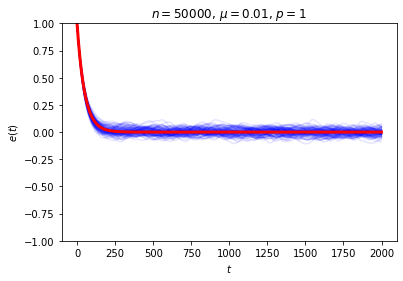
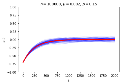
It’s possible to get a good picture of the typical behavior by just picking some initial conditions at random and looking at a graph of \(e\) over time. For each run, I randomly chose the markedness of each site and the color of each ball independently, so that each site is marked with probability \(\mu\) and each ball is black with probability \(p\). Each run lasted for 2000 time steps.

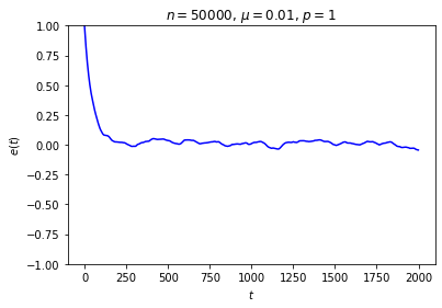
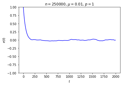
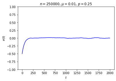
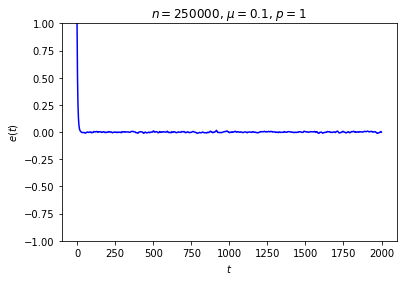
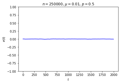
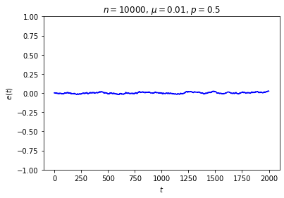
No matter where \(e\) starts, it seems to settle down to an “equilibrium value” of around zero — corresponding to equal numbers of black and white balls — with some fluctuations. These fluctuations are smaller when \(n\) is large, and \(e\) reaches equilibrium faster when \(\mu\) is closer to \(\frac12\).

This is somewhat similar to the situation with the gas in a box: in both cases, whether the system starts in equilibrium or not, once we start it running it moves toward equilibrium until the fluctuations drown out any difference between the current state and the equilibrium state, at which point there seems to be no evidence left of where we started. Our job is to explain this behavior.

The Initial Distribution

The first thing to note is that this equilibration doesn’t actually happen for every choice of initial conditions! It’s not that difficult to arrange the initial conditions so that \(e\) doesn’t go to 0, or doesn’t stabilize at all:

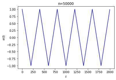
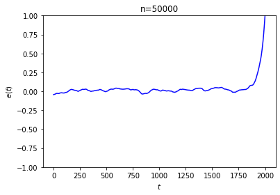
In the first run, we started with every ball black and marked every 200th site. The second run was generated by following a process like the one suggested in Loschmidt’s objection: we marked the sites randomly, started with every ball black, ran the system in reverse for 2000 steps, and took the result as our initial state.

We are forced to concede that we can’t expect this system to always approach equilibrium. This shouldn’t be too surprising: as the last example shows, Loschmidt’s reversibility objection applies to our system just as it applies to Boltzmann’s gas in a box.

Still, the examples we looked at earlier strongly suggest that, in some sense, a run with typical initial conditions will approach equilibrium. In order to make this case we’re going to have to decide exactly what “typical” means for us, that is, we’re going to have to choose some probability distribution for the initial conditions. It’s important to stress that this is a choice we’re making, and everything about the behavior we’re examining depends on it! We could certainly choose a distribution that makes initial conditions like the ones we just discussed highly probable, and it would then not be the case that a typical system approaches equilibrium.

The distribution we will use (which will not have this problem) depends on two parameters: \(p\), the probability that a ball starts out as black; and \(\mu\), the probability that a site starts out as marked. The probability distribution is uniquely determined by the choice of \(p\) and \(\mu\), together with the additional requirement that the initial states of all balls and sites are independent. This is, in fact, the distribution we drew our first examples from, and we will see that it exhibits exactly the behavior we’re looking for. (We will only ever consider \(\mu\le\frac12\), because we can convert the \(\mu>\frac12\) case into this one by switching the color of all balls at every time step.)

It will be helpful to introduce just a bit more notation:

• As before, write \(N_b(t)\) and \(N_w(t)\) for the number of black and white balls at time \(t\).
• Write \(\epsilon_i\) for the variable which is \(1\) if the \(i\)’th site is unmarked and \(-1\) if it is marked.
• Write \(\eta_i(t)\) for the variable which is \(1\) if, at time \(t\), the ball at the \(i\)’th site is black and \(-1\) if it’s white.

With this notation, we have \[e(t)=\frac1n\sum_{i=1}^n\eta_i(t),\] and the rule for moving time forward takes a simple form: \[\eta_i(t)=\epsilon_i\eta_{i-1}(t-1).\] (The expression “\(i-1\)” should be understood modulo \(n\), so that the indices wrap around from \(n\) to 1.)

We can use this to write \(e(t)\) just in terms of the initial conditions. We get that \[e(t)=\frac1n\sum_{i=1}^n\epsilon_i\epsilon_{i-1}\cdots\epsilon_{i-t+1}\eta_{i-t}(0).\] From here, it’s not that difficult to get a nice expression for the expected value of \(e(t)\). Because the \(\epsilon\)’s and \(\eta(0)\)’s are independent, the expected value of any product of them is the product of the expected values. As long as \(t\le n\), the \(\epsilon\)’s appearing in the product are all distinct, so we have \[\begin{aligned} \langle e(t)\rangle & = & \frac1n\sum_{i=1}^n\langle \epsilon_i\rangle\cdots\langle \epsilon_{i-t+1}\rangle\langle \eta_{i-t}(0)\rangle \\ & = & \frac1n\sum_{i=1}^n(1-2\mu)^t(2p-1) \\ & = & (1-2\mu)^t(2p-1).\end{aligned}\]

This is exactly the sort of thing we wanted to see, and it seems to give a decent answer to Loschmidt’s objection: on average, \(e(t)\) decays exponentially, so while trajectories in which it moves in the wrong direction aren’t impossible, they are unlikely. We can also see this in action by looking at the behavior of a large number of random trajectories. In each of the following graphs I superimposed 100 random trajectories in blue and the value of \(\langle e(t)\rangle\) we just computed in red:

Even though we seem to have shown that we get the sort of irreversible behavior we’re after on average, it can still be a little puzzling to work out “where the time symmetry went.” The answer is that the trajectory is determined by the rule for the dynamical system and the initial conditions, and while we never broke the symmetry in the rule, we did break the symmetry when we chose our initial condition.

Our distribution is stationary if we fix \(p=\frac12\), and in this case there is complete symmetry, since \(\langle e(t)\rangle\) starts and remains at 0. Again, trajectories that look like equilibration in reverse are possible, but very unlikely; it is much more probable for \(e(t)\) to just stay around 0 forever. But if we choose some other value of \(p\), impose the condition at \(t=0\), and then only look at positive values of \(t\), then we’ve broken the time symmetry. If we considered positive and negative times equally, we would approach equilibrium not as time goes forward per se, but as we get further away from the “unusual” (from the perspective of the stationary distribution) value of \(e(0)\).

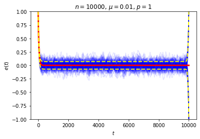
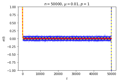
The astute reader may have noticed there’s a property of this system that we’ve been sweeping under the rug: what happens when \(t=n\), when each ball has made a full circuit around the ring? At this point every ball has seen all of the marked sites, so, depending on whether there’s an even or odd number of marked sites, we either have \(e(n)=e(0)\) or \(e(n)=-e(0)\). If we instead wait for \(2n\) time steps, the system will return to its original state no matter what. Either way, this is not the sort of equilibrium behavior we had in mind! We can see this directly if we look at a collection of random trajectories all the way out to \(t=n\):

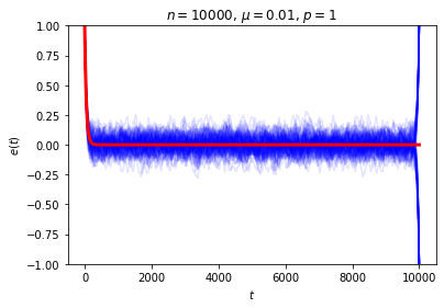
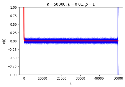
Our computation of the expected value of \(e(t)\) is correct even for \(t=n\), but focusing just on \(\langle e(n)\rangle\) is certainly misleading when the only reason it’s small is that it’s the average of a nearly equal number of \(1\)’s and \(-1\)’s. We can think of this phenomenon as a manifestation of Zermelo’s objection about recurrence: how can we talk about equilibration when the system returns to its original state every \(2n\) time steps?

Well, if “equilibration” is supposed to refer to a process that lasts forever, then we can’t. Still, there is some sort of approach to equilibrium going on, if only for times \(t\) much smaller than \(n\). We can get a better picture of the typical behavior of the system if we measure the variance of \(e(t)\) and not just its expected value. The computation is a bit more involved, but it uses the same set of ideas and I won’t go through it here. It’s a nice exercise if you’re so inclined. For simplicity we’ll just consider the case where \(p=1\), in which case the result is (take a deep breath): \[\mathrm{Var}(e(t)) = \begin{cases} 0 & t=0 \\ \frac1n\left(2\frac{1-(1-2\mu)^{2t}}{1-(1-2\mu)^2}-(2t-1)(1-2\mu)^{2t}-1\right) & 0<t\le \frac n2 \\ \frac1n\left(2\frac{1-(1-2\mu)^{2n-2t+2}}{1-(1-2\mu)^2}+(2t-n-1)(1-2\mu)^{2n-2t}-1\right)-(1-2\mu)^{2t} & \frac n2<t\le n \end{cases}\] The exact form of the variance is not especially important; there are only two features we need to notice. First, if \(t=n\), the variance is \(1-(1-2\mu)^n\), which is very close to 1, so indeed there is no reason to expect \(\langle e(n)\rangle\) to be a good estimate for \(e(n)\). But, more importantly, if we fix \(t\) and let \(n\) go to infinity, then we can see that the variance goes to zero. (Note that the expression inside the parentheses on the second line does not depend on \(n\).)

So, if \(n\) is very large and we only look at times \(t\) that are small compared to \(n\), most trajectories should stay very close to an exponential decay toward zero. We can again see this in action in our examples from above. Here we have drawn a dotted line at one standard deviation above and below the mean:

This resolution to Zermelo’s objection is very similar to Loschmidt’s. In both cases, the claim made in the objection is completely true, but we can still plausibly describe the system as approaching equilibrium so long as we are careful about what we mean.

Lessons for Real Physics

The Kac ring is, of course, much simpler than any actual physical system. This was advantangeous in one respect: it made it possible to actually prove everything we claimed about the approach to equilibrium. For more realistic models one usually just assumes that the system approaches equilibrium, or proves it under some simplifying assumptions. One might wonder just what we are supposed to conclude about real physics from this toy model, so it’s worth going through a few lessons that do in fact carry over.

• Equilibrium depends on the time scale. This shows up very clearly in our example: for times \(t\) much less than \(n\), we can profitably describe the system as approaching equilibrium, but around \(t=n\) we can’t. For us the thing that happens on that time scale was a Poincaré recurrence, but in the real world there can be plenty of other reasons to care about the time scale. Imagine a slightly cold, charged car battery sitting in a room-temperature garage. It might take just a couple of hours for the battery to warm up to the temperature of the room, but months or longer for it to lose its charge. After it has warmed up, is it “at equilibrium”? It depends on what processes you’re interested in. Richard Feynman famously defined equilibrium as when “all the fast things have happened but the slow things have not,” and this is much closer to the way the term is used in real life than anything more precise might be.

  As we mentioned before, recurrence times for real systems are truly enormous, far longer than current estimates of the age of the universe even for a box of gas that fits on a tabletop. But there are two more ways in which real physical systems get around the recurrence problem that didn’t show up for us.

  First, in general recurrence times depend on the initial state of the system, whereas our system always returned to its original state at \(t=2n\). So, in a realistic system, if we follow a large number of trajectories, then it will not actually be the case that all of them will return to their original state at once; at any given time at most a small fraction of them will have done so.

  Second, the Poincaré recurrence theorem only applies to closed systems, that is, systems which are isolated from their environment, and no realistic physical system has this property! In order to apply Zermelo’s objection in this case you would have to talk about the state of the system and its environment together, and the recurrence times involved will be that much larger.

• The prior distribution determines what behavior is “typical.” Statistical mechanics is the body of physics that seeks to describe thermodynamic behavior in terms of the statistical behavior of a system’s microscopic components. Everything about our analysis depended on the probability distribution we drew the initial conditions from, and as we discussed it is easy to imagine other distributions for which the approach to equilibrium is not the “typical” behavior. This is equally true for real-world statistical mechanics. Usually everyone agrees on which probability distributions to use, and their predictions match the results of experiments quite well, but this does not change the fact that all their computations depend on a choice of distribution. You can’t take the statistics out of statistical mechanics!
• Equilibrium depends on the choice of variables. Even if we restrict attention to the time scale on which the “approach to equilibrium” story makes sense, it was important to our analysis that the variable we were interested in was \(e(t)\); if, for example, we had just kept track of the color of the balls at the first and third sites, we wouldn’t have seen anything like equilibration.

  This feature of our model is meant to be a reflection of the fact that, for real systems, most of the details of the state are inaccessible and we can only measure a comparatively small number of “macroscopic variables”; this choice is usually constrained by what is easy to measure, but it is still choice. When we say that a real-world system has reached equilibrium, we mean that these macroscopic variables that we have chosen to keep track of seem to have stopped changing.

• Equilibration involves losing information. Another important aspect of the approach to equilibrium, closely connected to the irreversibility, is the loss of information. If we only track \(e(t)\), then once the number of black and white balls is approximately equal, any information about the initial value of \(e(t)\) is swamped by the “random” fluctuations, and so is essentially lost.

  Of course, the entire initial state is encoded, in a very opaque way, in the exact state at time \(t\); if we knew this exact state we could run time backwards and recover the initial value of \(e(t)\). Describing the state just in terms of \(e(t)\), then, throws out information, and not just information about the exact state but also information about previous values of \(e(t)\) itself. If you study statistical mechanics in more detail, you will learn that this is one way to think about the increase in entropy described by the second law of thermodynamics.

  Throwing out information in this way is only a good idea if it doesn’t much affect the future behavior of the system, and for our system this is again a question of time scales. Suppose we start the system with all white balls and after running until \(t=\frac34n\) the system is close to equilibrium. Are we free to forget everything except the value of \(e(t)\)? If we only run for a little while longer then this is fine, but if we run for \(\frac14n\) more time steps we’re in for a surprise!

  When analyzing real systems it’s often useful to “throw out” information in exactly this way, by only keeping track of the values of a small number of easily measurable variables, but information is also lost in another way that didn’t show up for us here. A real physical system is always interacting with its environment, and so, if we are only able to make detailed measurements of the system and not of the universe around it, we will also lose information over time just because of our ignorance of the details of this interaction.